20 · A linear CTR baseline and feature engineering
Chapter 18 remains the overview; this chapter isolates one question. The formal 200k experiment is preserved. Teaching runs use separate records in the shared registry.
Predict first: how do a constant prior and personalized probabilities differ?
CTR prediction maps impression features to click probabilities. A constant p equal to train CTR has no discrimination, but may have low ECE on rare-click tasks. Logistic regression maps an additive feature score to (0,1). One-hot encoding prevents anonymous hash magnitudes from implying ordered distances.
Fix the 40k prefix, partitions, C=1, optimization iterations, and numeric preprocessing. Change only whether the 26 categorical fields are included. All scores are on select; formal audit is not used for selection.
English companion. All instructional Markdown is translated. Experiment code, Chinese language examples, execution counts, and saved outputs remain as in the source edition; historical output text may therefore be Chinese. The initial setup cell anchors the working directory and Python import path for this companion's deeper folder; it does not change the experiment. Saved outputs are historical evidence, not a new run. Run from the top after preparing the required data and models.
# English companions live one directory deeper; keep the original experiment code unchanged.
from pathlib import Path as _TranslationPath
import os as _translation_os
import sys as _translation_sys
_translation_root = next((p for p in [_TranslationPath.cwd(), *_TranslationPath.cwd().parents]
                          if (p / "reclab").is_dir()), None)
if _translation_root is None:
    raise RuntimeError("Open this notebook from inside the Search Recommendation Ads Lab checkout.")
_translation_os.chdir(_translation_root)
if str(_translation_root) not in _translation_sys.path:
    _translation_sys.path.insert(0, str(_translation_root))
from pathlib import Path
import sys
ROOT=Path.cwd()
if not (ROOT/'reclab').is_dir(): ROOT=ROOT.parent
sys.path.insert(0,str(ROOT))
import numpy as np
import pandas as pd
import matplotlib.pyplot as plt
from IPython.display import display
from reclab.ads import latest, load_data, split_groups, NUM, CAT, FEATURES
from reclab.paths import ARTIFACTS
from reclab.probability import evaluate
preview=ARTIFACTS/'notebook-previews';preview.mkdir(parents=True,exist_ok=True)
frame,_=load_data(40000);masks,_=split_groups(frame);y=frame.label.to_numpy()
prior=np.full(int(masks['select'].sum()),y[masks['train']].mean())
print('Input:',frame[FEATURES].shape,'label:',y.shape)
print('Train prior, select evaluation:',{k:v for k,v in evaluate(y[masks['select']],prior).items() if k!='reliability'})
Saved notebook output · not executed on this page
Input: (40000, 39) label: (40000,)
Train prior, select evaluation: {'n': 6006, 'positives': 194, 'click_rate': 0.032301032301032304, 'mean_probability': 0.030739193606974205, 'auc': 0.5, 'logloss': 0.14269226135422958, 'brier': 0.03126011495342623, 'ece': 0.0015618386940580986}
From inputs to a design matrix
Signed log1p preserves the direction of negative values while compressing long tails. Follow with train-median imputation, missingness indicators, and standardization. Categories use sparse one-hot encoding with at most 128 categories; the same encoder handles rare/unseen values. Final dimension is not 39: inspect shape and sparse storage.
Inspect the numeric design matrix first. Predict how many missingness-indicator columns are added. Some columns are never missing on train, so the increase is not necessarily 13.
from sklearn.pipeline import make_pipeline
from sklearn.preprocessing import FunctionTransformer,StandardScaler
from sklearn.impute import SimpleImputer
from reclab.ads import signed_log
numeric=make_pipeline(FunctionTransformer(signed_log),SimpleImputer(strategy='median',add_indicator=True),StandardScaler())
z=numeric.fit_transform(frame.loc[masks['train'],NUM])
print('Raw numeric:',(int(masks['train'].sum()),13),'transformed:',z.shape)
assert np.isfinite(z).all()
print('Scale learned on train; select is transform-only:',numeric.transform(frame.loc[masks['select'],NUM]).shape)
Saved notebook output · not executed on this page
Raw numeric: (22024, 13) transformed: (22024, 24)
Scale learned on train; select is transform-only: (6006, 24)
Run real training: add only categorical features
The shared teaching trainer fits both arms independently. Each execution creates a new ads record, saves local coefficients and select predictions, and retains failures. It never replaces the formal 200k model. It should take seconds on the reference machine; use actual local wall time.
Write your expected directions for AUC and logloss, then run. Any improvement applies only to this prefix and feature budget.
from reclab.ads_teaching import workshop
run_id,comparison=workshop('linear_features')
print('Shared workshop run:',run_id,'shapes:',comparison['shapes'])
table=pd.DataFrame([{'method':r['method'],'dimension':r['features'],'seconds':r['fit_seconds'],'iterations':r['iterations'],**{k:r['select'][k] for k in ['auc','logloss','brier','ece']}} for r in comparison['rows']])
display(table)
assert all(r['iterations']<300 for r in comparison['rows'])
Saved notebook output · not executed on this page
Shared workshop run: 20261030T130907-22ac6037 shapes: {'raw': [40000, 39], 'train': 22024, 'select': 6006}
| method | dimension | seconds | iterations | auc | logloss | brier | ece | |
|---|---|---|---|---|---|---|---|---|
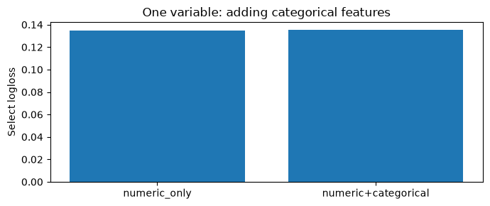
| 0 | numeric_only | 24 | 0.059206 | 14 | 0.707051 | 0.134451 | 0.030668 | 0.001666 |
| 1 | numeric+categorical | 2470 | 0.814952 | 108 | 0.721102 | 0.135359 | 0.031107 | 0.008736 |
Interpret coefficients with their units
The linear model is additive in log-odds. A standardized numeric coefficient corresponds to one training standard deviation; a one-hot coefficient is a relative shift conditional on the encoding. Missingness indicators and category encoding mean a large coefficient is not evidence that a real factor causes clicks. Anonymous data cannot justify user profiling.
Inspect coefficient shape, nonzero count, and probability range in the local NPZ. Only aggregate norms are shown here; weights stay out of Git.
folder=ARTIFACTS/'experiments/ads'/run_id
for row in comparison['rows']:
    weights=np.load(folder/(row['method']+'.npz'),allow_pickle=False)
    print(row['method'],'coef shape:',weights['coef'].shape,'L2 norm:',float(np.linalg.norm(weights['coef'])),
          'probability range:',float(weights['select_probability'].min()),float(weights['select_probability'].max()))
fig,ax=plt.subplots(figsize=(7,3));ax.bar(table.method,table.logloss)
ax.set(ylabel='Select logloss',title='One variable: adding categorical features');fig.tight_layout();fig.savefig(preview/'20_linear.png',dpi=130);plt.show()
Saved notebook output · not executed on this page
numeric_only coef shape: (1, 24) L2 norm: 0.5670679800150403 probability range: 0.0010747912904707244 0.24311326416319087
numeric+categorical coef shape: (1, 2470) L2 norm: 16.457663076525826 probability range: 4.10356476796253e-05 0.7478277943321489
<Figure size 700x300 with 1 Axes>
A one-variable exercise and interpretation
Keep features fixed and change only C in a temporary model. Predict how stronger regularization changes probability distributions. The loss stress test below changes confidence only; it is not a retrained model. Shrinking p toward the train prior may preserve discrimination while changing probability loss.
Equal AUC does not imply equal logloss. Improving one metric does not establish online gains. A genuine C comparison should extend the shared trainer's configuration, use select, and preserve a new independent final audit.
saved=np.load(folder/'numeric+categorical.npz',allow_pickle=False)
p=saved['select_probability'];rate=float(y[masks['train']].mean())
alpha=.5  # Exercise: change only this shrinkage factor.
shrunk=alpha*p+(1-alpha)*rate
for name,prob in [('original',p),('shrink_to_prior',shrunk)]:
    r=evaluate(y[masks['select']],prob);print(name,{k:r[k] for k in ['auc','logloss','brier']})
print('This is a controlled probability transform, not a retrained regularization experiment.')
Saved notebook output · not executed on this page
original {'auc': 0.7211022697440772, 'logloss': 0.13535924760121054, 'brier': 0.031106683422217875}
shrink_to_prior {'auc': 0.7211022697440772, 'logloss': 0.13363860416569606, 'brier': 0.030527528460338932}
This is a controlled probability transform, not a retrained regularization experiment.