22 · Probability scores, reliability, and calibration audit
Chapter 18 remains the overview; this chapter isolates one question. The formal 200k experiment is preserved. Teaching runs use separate records in the shared registry.
Predict first: does correct ordering imply accurate probabilities?
AUC measures positive/negative ordering; logloss strongly penalizes overconfident mistakes; Brier is squared probability error. They answer different questions. Calibration requires observed click rates near predicted probabilities to match; a visually attractive reliability curve is insufficient.
Use saved real per-impression predictions from the formal experiment; details stay local. Fix base model and samples, inspect shapes, then refit the same prespecified sigmoid on independent calibration and verify audit results. Do not add audit-based selection.
English companion. All instructional Markdown is translated. Experiment code, Chinese language examples, execution counts, and saved outputs remain as in the source edition; historical output text may therefore be Chinese. The initial setup cell anchors the working directory and Python import path for this companion's deeper folder; it does not change the experiment. Saved outputs are historical evidence, not a new run. Run from the top after preparing the required data and models.
# English companions live one directory deeper; keep the original experiment code unchanged.
from pathlib import Path as _TranslationPath
import os as _translation_os
import sys as _translation_sys
_translation_root = next((p for p in [_TranslationPath.cwd(), *_TranslationPath.cwd().parents]
                          if (p / "reclab").is_dir()), None)
if _translation_root is None:
    raise RuntimeError("Open this notebook from inside the Search Recommendation Ads Lab checkout.")
_translation_os.chdir(_translation_root)
if str(_translation_root) not in _translation_sys.path:
    _translation_sys.path.insert(0, str(_translation_root))
from pathlib import Path
import sys
ROOT=Path.cwd()
if not (ROOT/'reclab').is_dir(): ROOT=ROOT.parent
sys.path.insert(0,str(ROOT))
import numpy as np
import pandas as pd
import matplotlib.pyplot as plt
from IPython.display import display
from reclab.ads import latest, load_data, split_groups, NUM, CAT, FEATURES
from reclab.paths import ARTIFACTS
from reclab.probability import evaluate
preview=ARTIFACTS/'notebook-previews';preview.mkdir(parents=True,exist_ok=True)
receipt,result=latest();folder=ARTIFACTS/'experiments/ads'/receipt['run_id']
data=np.load(folder/'predictions.npz',allow_pickle=False)
y=data['label'];raw=data[result['selected_base']];cal=data['split']==2;audit=data['split']==3
print('Probability vector:',raw.shape,'calibration:',int(cal.sum()),'audit:',int(audit.sum()))
print('Actual audit positives:',int(y[audit].sum()))
Saved notebook output · not executed on this page
Probability vector: (200000,) calibration: 30153 audit: 29928
Actual audit positives: 992
Calculate probability losses by hand
For y∈{0,1}, logloss=−[y log(p)+(1−y)log(1−p)], and Brier=(p−y)². The two samples below are explicitly constructed tensors. At p=.25/.75, compute −log(.75) and .0625. More extreme probabilities with the same ordering may help when correct and cost more when wrong.
Write the prediction, then execute assertions. This verifies implementation, not real evaluation.
toy_y=np.array([0,1]);toy_p=np.array([.25,.75])
r=evaluate(toy_y,toy_p)
assert np.isclose(r['logloss'],-np.log(.75)) and np.isclose(r['brier'],.0625)
for name,p in [('moderate',toy_p),('confident_correct',np.array([.01,.99])),('confident_wrong',np.array([.99,.01]))]:
 print(name,{k:evaluate(toy_y,p)[k] for k in ['auc','logloss','brier']})
Saved notebook output · not executed on this page
moderate {'auc': 1.0, 'logloss': 0.2876820724517809, 'brier': 0.0625}
confident_correct {'auc': 1.0, 'logloss': 0.01005033585350145, 'brier': 0.00010000000000000014}
confident_wrong {'auc': 0.0, 'logloss': 4.605170185988091, 'brier': 0.9801}
Actually refit the same sigmoid to the same base model
The input is an [Ncal,1] matrix of logit(p), using calibration labels only. LogisticRegression C=1e6 is a prespecified approximately unregularized map, not selected on audit. Positive slope preserves order; negative slope reverses it, so unchanged AUC must not be assumed. This run should match saved predictions.
Do not choose sigmoid deployment from a slight audit improvement: the paired interval crosses zero, so retain uncertainty.
from sklearn.linear_model import LogisticRegression
from reclab.ads import logit
mapper=LogisticRegression(C=1e6,solver='lbfgs',max_iter=200).fit(logit(raw[cal])[:,None],y[cal])
p=mapper.predict_proba(logit(raw[audit])[:,None])[:,1]
assert np.allclose(p,data['selected_sigmoid'][audit],atol=1e-10)
for name,prob in [('raw',raw[audit]),('refit_fixed_sigmoid',p),('stored_isotonic',data['selected_isotonic'][audit])]:
 r=evaluate(y[audit],prob);print(name,{k:r[k] for k in ['auc','logloss','brier','ece']})
print(result['paired_sigmoid'])
Saved notebook output · not executed on this page
raw {'auc': 0.7063291304168487, 'logloss': 0.1360293933130953, 'brier': 0.031221289955195537, 'ece': 0.001738314050279206}
refit_fixed_sigmoid {'auc': 0.7063291304168487, 'logloss': 0.13596808940352492, 'brier': 0.031218897836043032, 'ece': 0.0011488903239790385}
stored_isotonic {'auc': 0.7030639468805462, 'logloss': 0.1364371767207884, 'brier': 0.0313022514243036, 'ece': 0.0011632039192470336}
{'calibrated_minus_raw_logloss': -6.130390957040765e-05, 'iid_row_bootstrap_95': [-0.00016953362229380587, 6.253575759107997e-05], 'replicates': 300, 'limitation': 'conditional on fitted models; repeated/related rows and one shard limit independence and generalization'}
Change one variable: ECE bin count
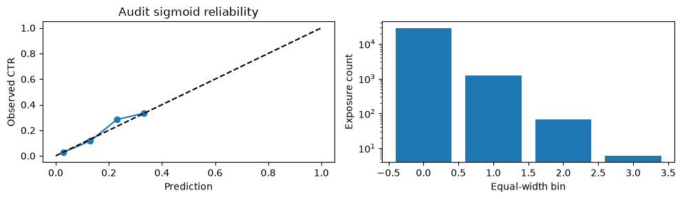
ECE is not a proper scoring rule; bin boundaries and sample size affect it. Predict the effect of changing five bins to 20, then calculate with identical predictions and labels. Inspect counts: one or two samples in a high-probability bin cannot establish a stable segment pattern.
Do not choose bins or models by audit ECE. This is metric-sensitivity analysis; formal reporting retains the prespecified ten bins.
display(pd.DataFrame([{'bins':b,'ece':evaluate(y[audit],p,bins=b)['ece']} for b in [5,10,20]]))
r=evaluate(y[audit],p,bins=10);bins=pd.DataFrame(r['reliability']);display(bins)
fig,axes=plt.subplots(1,2,figsize=(10,3));axes[0].plot(bins.mean_probability,bins.click_rate,'o-');axes[0].plot([0,1],[0,1],'k--')
axes[0].set(xlabel='Prediction',ylabel='Observed CTR',title='Audit sigmoid reliability');axes[1].bar(bins.bin,bins['count']);axes[1].set(xlabel='Equal-width bin',ylabel='Exposure count',yscale='log')
fig.tight_layout();fig.savefig(preview/'22_calibration.png',dpi=130);plt.show()
Saved notebook output · not executed on this page
| bins | ece | |
|---|---|---|
| 0 | 5 | 0.001149 |
| 1 | 10 | 0.001149 |
| 2 | 20 | 0.001376 |
| bin | count | mean_probability | click_rate | |
|---|---|---|---|---|
| 0 | 0 | 28639 | 0.029438 | 0.028947 |
| 1 | 1 | 1216 | 0.130528 | 0.116776 |
| 2 | 2 | 67 | 0.230115 | 0.283582 |
| 3 | 3 | 6 | 0.330736 | 0.333333 |
<Figure size 1000x300 with 2 Axes>
Segments and conclusion boundaries
Unseen-category and missingness segments have different click base rates. Absolute logloss alone cannot establish which segment the model serves worse. Inspect count, base rate, mean prediction, and loss together. Anonymous fields do not permit demographic fairness evaluation, and undisclosed sampling rates prevent recovering population CTR.
Exercise: change one real sample's input in the workbench and inspect its probability. An input counterfactual is not a real causal effect. Segment aggregates below remain from the prespecified audit; no new selection is performed.
display(pd.DataFrame([{'segment':s['segment'],'n':s['raw']['n'],'CTR':s['raw']['click_rate'],'raw_mean':s['raw']['mean_probability'],'sigmoid_mean':s['sigmoid']['mean_probability'],'raw_loss':s['raw']['logloss'],'sigmoid_loss':s['sigmoid']['logloss']} for s in result['segments']]))
print('Conclusion: small sigmoid loss change is uncertain; isotonic negative result remains. Population calibration is unidentified.')
Saved notebook output · not executed on this page
| segment | n | CTR | raw_mean | sigmoid_mean | raw_loss | sigmoid_loss | |
|---|---|---|---|---|---|---|---|
| 0 | low_numeric_missing | 17016 | 0.036495 | 0.035931 | 0.037111 | 0.147043 | 0.146935 |
| 1 | high_numeric_missing | 12912 | 0.028733 | 0.028715 | 0.030027 | 0.121515 | 0.121515 |
| 2 | any_unseen_category | 11668 | 0.035996 | 0.034161 | 0.035395 | 0.146929 | 0.146712 |
| 3 | all_categories_seen | 18260 | 0.031325 | 0.031960 | 0.033198 | 0.129065 | 0.129103 |
Conclusion: small sigmoid loss change is uncertain; isotonic negative result remains. Population calibration is unidentified.