33 · Optimization, capacity, and generalization
Foundations path: 31 → 32 → 33 → 34, then choose search, ads, or recommendation.
Scope: constructed small-array mechanism experiments on CPU; no real logs, formal model training, or business-impact claims.
For each section: predict → change one variable → run → explain. Execute from the beginning first; after edits, rerun affected downstream cells.
English companion. All instructional Markdown is translated. Experiment code, Chinese language examples, execution counts, and saved outputs remain as in the source edition; historical output text may therefore be Chinese. The initial setup cell anchors the working directory and Python import path for this companion's deeper folder; it does not change the experiment. Saved outputs are historical evidence, not a new run. Run from the top after preparing the required data and models.
# English companions live one directory deeper; keep the original experiment code unchanged.
from pathlib import Path as _TranslationPath
import os as _translation_os
import sys as _translation_sys
_translation_root = next((p for p in [_TranslationPath.cwd(), *_TranslationPath.cwd().parents]
                          if (p / "reclab").is_dir()), None)
if _translation_root is None:
    raise RuntimeError("Open this notebook from inside the Search Recommendation Ads Lab checkout.")
_translation_os.chdir(_translation_root)
if str(_translation_root) not in _translation_sys.path:
    _translation_sys.path.insert(0, str(_translation_root))
A controlled starting point for optimization
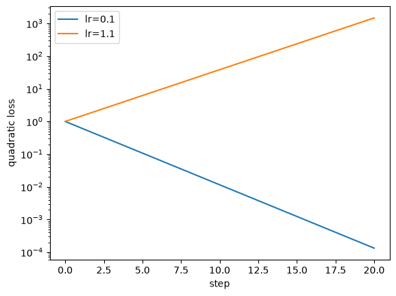
Apply gradient descent to L(w)=w². This isolates learning rate; it says nothing about data generalization.
import numpy as np
import matplotlib.pyplot as plt
from reclab.learning.foundations import quadratic_descent, polynomial_fit
curves = {lr: quadratic_descent(lr) for lr in [0.1, 1.1]}
assert curves[0.1][-1]**2 < curves[0.1][0]**2
assert curves[1.1][-1]**2 > curves[1.1][0]**2
for lr, values in curves.items():
    plt.semilogy(np.square(values), label=f'lr={lr}')
plt.xlabel('step'); plt.ylabel('quadratic loss'); plt.legend(); plt.show()
Saved notebook output · not executed on this page
<Figure size 640x480 with 1 Axes>
Fixed constructed training and selection sets
The true function is linear; training labels have fixed noise. Selection samples use different coordinates from the same function. This is not a real-world distribution. Predict the higher-order model's training error.
train_x = np.linspace(-1, 1, 10)
noise = np.array([.1,-.2,.15,-.1,.2,-.15,.05,.12,-.18,.1])
train_y = 1 + 2*train_x + noise
select_x = np.linspace(-.95, .95, 80)
select_y = 1 + 2*select_x
assert train_x.shape == train_y.shape == (10,)
Change only polynomial degree
Use the same training points and least-squares solver to compare degree 1 and 9. Selection labels do not fit coefficients.
fits = {degree: polynomial_fit(train_x, train_y, select_x, degree) for degree in [1, 9]}
errors = {d: (np.mean((a-train_y)**2), np.mean((b-select_y)**2)) for d,(a,b) in fits.items()}
assert errors[9][0] < errors[1][0]
assert errors[9][1] > errors[1][1]
print('degree: (train MSE, select MSE)', errors)
Saved notebook output · not executed on this page
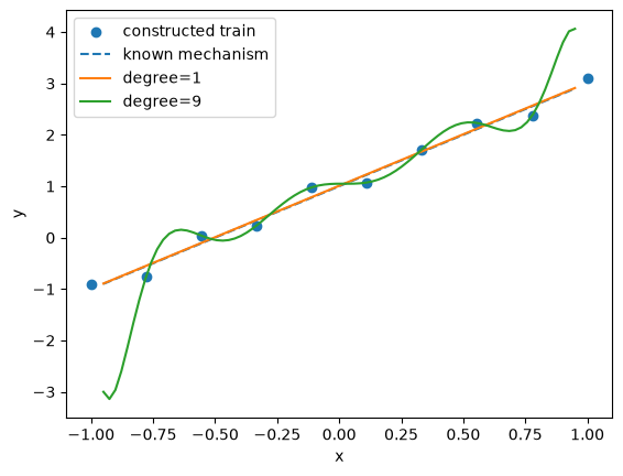
degree: (train MSE, select MSE) {1: (np.float64(0.02034654545454546), np.float64(8.285834370750043e-05)), 9: (np.float64(6.981254151602715e-28), np.float64(0.35380856429606694))}
Inspect local failure and evaluation boundaries
Plot the same predictions. Once selection data chooses degree, it can no longer be called an unseen audit set.
plt.scatter(train_x, train_y, label='constructed train')
plt.plot(select_x, select_y, '--', label='known mechanism')
for degree, (_, prediction) in fits.items():
    plt.plot(select_x, prediction, label=f'degree={degree}')
plt.xlabel('x'); plt.ylabel('y'); plt.legend(); plt.show()
Saved notebook output · not executed on this page
<Figure size 640x480 with 1 Axes>
Explain
Why does lower training error fail to reduce selection error? How would you preserve a genuinely independent final evaluation set? This example holds for fixed noise. Predict before changing the noise seed; do not turn one result into a universal law.
In the next cell, record your prediction, actual result, reason for any difference, and applicability limits. Keep failed results.
reflection = {'预测': '', '结果': '', '解释与边界': ''}
reflection
Saved notebook output · not executed on this page
{'预测': '', '结果': '', '解释与边界': ''}