13 · Negative sampling, BPR, and LightGCN
Goal
Sample (user, positive, unknown) triples yourself, inspect graph-propagation tensors, and run a small training job.
Artificial tensors are explicitly labeled as mechanism demonstrations; training uses real t1 histories.
Setup
Model and training loop · Original winning model.
English companion. All instructional Markdown is translated. Experiment code, Chinese language examples, execution counts, and saved outputs remain as in the source edition; historical output text may therefore be Chinese. The initial setup cell anchors the working directory and Python import path for this companion's deeper folder; it does not change the experiment. Saved outputs are historical evidence, not a new run. Run from the top after preparing the required data and models.
# English companions live one directory deeper; keep the original experiment code unchanged.
from pathlib import Path as _TranslationPath
import os as _translation_os
import sys as _translation_sys
_translation_root = next((p for p in [_TranslationPath.cwd(), *_TranslationPath.cwd().parents]
                          if (p / "reclab").is_dir()), None)
if _translation_root is None:
    raise RuntimeError("Open this notebook from inside the Search Recommendation Ads Lab checkout.")
_translation_os.chdir(_translation_root)
if str(_translation_root) not in _translation_sys.path:
    _translation_sys.path.insert(0, str(_translation_root))
from pathlib import Path
import sys, json, inspect
ROOT = Path.cwd()
if not (ROOT / "reclab").is_dir():
    ROOT = ROOT.parent
sys.path.insert(0, str(ROOT))
import numpy as np
import pandas as pd
import matplotlib.pyplot as plt
from IPython.display import display, Code
from reclab.competition import data
from reclab.competition.teaching import load_run, style, bar_scores
style()
pd.set_option("display.max_columns", 12)
pd.set_option("display.max_rows", 40)
run, rows, features = load_run()
print("实际训练快照:", run.name)
Saved notebook output · not executed on this page
实际训练快照: 20261030T115556803593-cloud-restore
Step 1 · Sampling rules encode model assumptions
First sample a user uniformly, then a positive uniformly from that user's known history, and reject-sample a negative from unseen items.
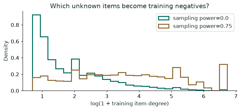
These "negatives" are unknown items and may include future favorites. negative_power=.75 samples in proportion to popularity raised to .75; it optimizes a different distribution from uniform sampling.
from reclab.competition.data import encode
from reclab.competition.graph import NegativeSampler, normalized_graph, LightGCN, GraphConfig, train_graph, graph_score
import torch
real = data.corpus(["t1"])
users, items, history = encode(real)
history.data[:] = 1
draws = {}
for power in [0., .75]:
    sampler = NegativeSampler(history, power=power, seed=2022)
    u, p, n = sampler.sample(20000)
    assert sampler.is_known(u, p).all() and not sampler.is_known(u, n).any()
    popularity = np.asarray(history.sum(axis=0)).ravel()
    draws[power] = popularity[n]
    print("power:", power, "负例平均训练热度:", round(float(popularity[n].mean()), 2))
display(pd.DataFrame({"user": users[u[:5]], "positive": items[p[:5]], "sampled_unknown": items[n[:5]]}))
Saved notebook output · not executed on this page
power: 0.0 负例平均训练热度: 17.28
power: 0.75 负例平均训练热度: 121.4
| user | positive | sampled_unknown | |
|---|---|---|---|
| 0 | t1U1007037 | P1007562 | P1026949 |
| 1 | t1U1002463 | P1009950 | P1032560 |
| 2 | t1U1007458 | P1018990 | P1022155 |
| 3 | t1U1000925 | P1004032 | P1003943 |
| 4 | t1U1001876 | P1004147 | P1009057 |
fig, ax = plt.subplots(figsize=(8, 3))
for power, values in draws.items():
    ax.hist(np.log1p(values), bins=25, histtype="step", linewidth=2, density=True, label=f"sampling power={power}")
ax.set(xlabel="log(1 + training item degree)", ylabel="Density", title="Which unknown items become training negatives?")
ax.legend(); plt.show()
Saved notebook output · not executed on this page
<Figure size 880x330 with 1 Axes>
Step 2 · Check propagation on constructed tensors
Only three users and four items appear below: a constructed mechanism demonstration.
Adjacency matrix A connects users and items on opposite sides. Propagate after normalization by D^-1/2 A D^-1/2.
The final representation averages layers 0 through L, without an MLP, nonlinearities, or additional feature transformations.
from scipy import sparse
toy = sparse.csr_matrix([[1,1,0,0], [0,1,1,0], [0,0,1,1]], dtype=np.float32)
graph = normalized_graph(toy)
torch.manual_seed(2022)
net = LightGCN(3, 4, dim=8, layers=2)
user_vectors, item_vectors = net.propagate(graph)
print("邻接矩阵", tuple(graph.shape), "用户向量", tuple(user_vectors.shape), "商品向量", tuple(item_vectors.shape))
u0, p0, n0 = torch.tensor([0,1]), torch.tensor([0,1]), torch.tensor([3,0])
loss, reg = net.bpr_loss(graph, u0, p0, n0)
loss.backward()
print("BPR:", float(loss.detach()), "ego L2:", float(reg.detach()))
print("Embedding gradient norm:", float(net.item_embedding.weight.grad.norm()))
assert torch.isfinite(net.item_embedding.weight.grad).all()
Saved notebook output · not executed on this page
邻接矩阵 (7, 7) 用户向量 (3, 8) 商品向量 (4, 8)
BPR: 0.6874470710754395 ego L2: 0.1299145221710205
Embedding gradient norm: 0.041438326239585876
Step 3 · Edit code and run real training
This cell actually trains a model without overwriting the main experiment. Start with 16 dimensions and four epochs to inspect the full process in tens of seconds on the reference machine.
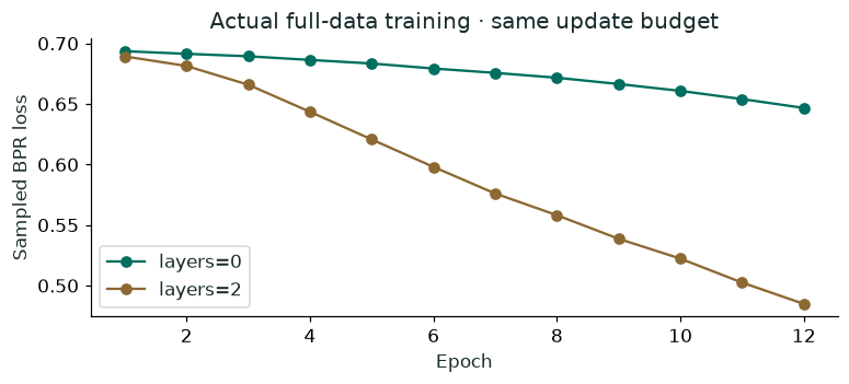
Set layers=0 for an MF comparison at the same training budget; set negative_power=.75 to investigate sampling.
Lower BPR loss does not guarantee better candidate rankings. After editing the .py file, execute the reload cell, then rerun training.
import importlib
import reclab.competition.graph as graph_module
importlib.reload(graph_module)
CONFIG = graph_module.GraphConfig(dim=16, layers=2, epochs=4, steps_per_epoch=2, negative_power=0.)
sandbox = graph_module.train_graph(real, CONFIG)
target = data.candidates("t1")
sandbox_scores = graph_module.graph_score(sandbox, target)
from reclab.competition.metrics import evaluate
display(evaluate(target, sandbox_scores))
# 保存到本轮 Notebook 沙盒文件,和主实验分开。
from datetime import datetime, timezone
sandbox_path = data.OUTPUT / "experiments" / (datetime.now(timezone.utc).strftime("%Y%m%dT%H%M%S%f") + "-graph")
sandbox_path.mkdir(parents=True)
torch.save({"state_dict": sandbox["model"].state_dict(), "config": sandbox["config"]}, sandbox_path / "model.pt")
(sandbox_path / "trace.json").write_text(json.dumps(sandbox["trace"], indent=2))
print("沙盒保存:", sandbox_path)
Saved notebook output · not executed on this page
LightGCN layers=2 epoch=1: bpr=0.69083
LightGCN layers=2 epoch=2: bpr=0.68599
LightGCN layers=2 epoch=3: bpr=0.67694
LightGCN layers=2 epoch=4: bpr=0.66325
| market | users | ndcg10 | hr10 | |
|---|---|---|---|---|
| 0 | t1 | 2697 | 0.428107 | 0.536522 |
| 1 | combined | 2697 | 0.428107 | 0.536522 |
沙盒保存: /Users/lynnlee/Documents/Codex/2026-10-30/task/soutui-lab/artifacts/xmrec/experiments/20261030T115936874041-graph
Step 4 · Revisit the main experiment and resource differences
The main experiment uses the complete five-market corpus; the plot shows saved curves from the actual run. The winning paper uses 2,048 dimensions, four layers, learning rate .001, and dropout .4. The local version uses 32 dimensions, two layers, learning rate .01, no dropout, and only a small number of large-batch updates. Numerical agreement verifies core formulas, not an identical training recipe or final score.
trace = json.loads((run / "graph_trace.json").read_text())
fig, ax = plt.subplots(figsize=(8, 3))
for layers, values in trace.items():
    t = pd.DataFrame(values)
    ax.plot(t.epoch, t.bpr, marker="o", label=f"layers={layers}")
ax.set(xlabel="Epoch", ylabel="Sampled BPR loss", title="Actual full-data training · same update budget")
ax.legend(); plt.show()
display(pd.Series(json.loads((run / "config.json").read_text())["graph"]))
Saved notebook output · not executed on this page
<Figure size 880x330 with 1 Axes>
dim                   32.0000
layers                 2.0000
epochs                12.0000
steps_per_epoch        3.0000
batch_size         32768.0000
lr                     0.0100
decay                  0.0001
negative_power         0.0000
seed                2022.0000
threads                4.0000
dtype: float64
Check and continue
Why can loss become very small while nDCG on the 100 official candidates stays poor?