18 · One system: real click probabilities and simulated ad decisions
Predict → change one variable → execute → explain. Reuse the same experiment records, download verifier, FastAPI, and workbench.
The real component is official Criteo impression/click data. The simulated component is a separately generated second-price market. They have no demonstrated real-revenue or causal connection. Positive/negative sampling rates are unknown; probabilities apply only to the public sample distribution.
Predict first: must a more complex tree outperform a linear model? Must calibration improve logloss? Does a tiny ECE make a constant prior useful?
English companion. All instructional Markdown is translated. Experiment code, Chinese language examples, execution counts, and saved outputs remain as in the source edition; historical output text may therefore be Chinese. The initial setup cell anchors the working directory and Python import path for this companion's deeper folder; it does not change the experiment. Saved outputs are historical evidence, not a new run. Run from the top after preparing the required data and models.
# English companions live one directory deeper; keep the original experiment code unchanged.
from pathlib import Path as _TranslationPath
import os as _translation_os
import sys as _translation_sys
_translation_root = next((p for p in [_TranslationPath.cwd(), *_TranslationPath.cwd().parents]
                          if (p / "reclab").is_dir()), None)
if _translation_root is None:
    raise RuntimeError("Open this notebook from inside the Search Recommendation Ads Lab checkout.")
_translation_os.chdir(_translation_root)
if str(_translation_root) not in _translation_sys.path:
    _translation_sys.path.insert(0, str(_translation_root))
from pathlib import Path
import sys
ROOT=Path.cwd()
if not (ROOT/'reclab').is_dir(): ROOT=ROOT.parent
sys.path.insert(0,str(ROOT))
import numpy as np
import pandas as pd
import matplotlib.pyplot as plt
from reclab.ads import latest
from reclab.paths import ARTIFACTS
receipt, result=latest()
folder=ARTIFACTS/'experiments/ads'/receipt['run_id']
print('Shared run:', receipt['run_id'])
print(result['scope'])
display(pd.DataFrame(result['splits']).T)
assert sum(x['n'] for x in result['splits'].values())==receipt['config']['rows']
print('Feature duplicate rows:',result['feature_duplicate_rows'])
print('Grouping uses features only; no temporal/user holdout is claimed.')
Saved notebook output · not executed on this page
Shared run: 20261030T125738-f82b6582
Criteo official sampled click logs: first 200,000 rows of one 766,864-row parquet shard (2015-02-15). Real CTR task on a subsampled distribution. Auction is a separate synthetic market.
| n | positives | click_rate | unique_feature_groups | |
|---|---|---|---|---|
| train | 109935.0 | 3614.0 | 0.032874 | 109934.0 |
| select | 29984.0 | 1016.0 | 0.033885 | 29984.0 |
| calibration | 30153.0 | 1023.0 | 0.033927 | 30153.0 |
| audit | 29928.0 | 992.0 | 0.033146 | 29928.0 |
Feature duplicate rows: 1
Grouping uses features only; no temporal/user holdout is claimed.
Compare real probabilities first, using appropriate metrics
AUC measures discrimination; logloss and Brier measure probability quality. ECE uses ten equal-width bins. A constant prior can have low ECE when clicks are rare, so ECE alone cannot select a model. Encoders fit on train only. Select chooses only between 80 and 160 trees; calibration independently fits sigmoid and isotonic maps. Audit does not choose models; the linear model remains an independent baseline.
Run the next cell and inspect negative results. The complete coefficient table is local at linear_coefficients.csv; weights are not uploaded.
summary=pd.DataFrame([{'method':r['method'],**{k:r['audit'][k] for k in ['auc','logloss','brier','ece']},'fit_seconds':r['fit_seconds']} for r in result['rows']])
display(summary.round(6))
print('GBDT family selected by select logloss:',result['selected_base'])
fig,axes=plt.subplots(1,2,figsize=(11,4))
for row in result['rows']:
    if row['method'] in [result['selected_base'],'selected_sigmoid','selected_isotonic']:
        bins=row['audit']['reliability']
        axes[0].plot([b['mean_probability'] for b in bins],[b['click_rate'] for b in bins],marker='o',label=row['method'])
axes[0].plot([0,1],[0,1],'k--',alpha=.5)
axes[0].set(xlabel='Mean predicted probability',ylabel='Observed click rate',title='Audit reliability: sparse high bins')
axes[0].legend(fontsize=8)
axes[1].barh(summary.method,summary.logloss)
axes[1].set(xlabel='Audit logloss (lower is better)',title='All baselines and negative results')
fig.tight_layout()
preview=ROOT/'artifacts/notebook-previews';preview.mkdir(parents=True,exist_ok=True)
fig.savefig(preview/'18_probability.png',dpi=140)
plt.show()
Saved notebook output · not executed on this page
| method | auc | logloss | brier | ece | fit_seconds | |
|---|---|---|---|---|---|---|
| 0 | train_prior | 0.500000 | 0.145515 | 0.032048 | 0.000272 | 0.000000 |
| 1 | linear_onehot | 0.721468 | 0.135423 | 0.031193 | 0.004382 | 4.102396 |
| 2 | gbdt_80 | 0.706329 | 0.136029 | 0.031221 | 0.001738 | 0.555461 |
| 3 | gbdt_160 | 0.703035 | 0.137404 | 0.031358 | 0.005350 | 0.932227 |
| 4 | selected_sigmoid | 0.706329 | 0.135968 | 0.031219 | 0.001149 | 0.008740 |
| 5 | selected_isotonic | 0.703064 | 0.136437 | 0.031302 | 0.001163 | 0.006879 |
GBDT family selected by select logloss: gbdt_80
<Figure size 1100x400 with 2 Axes>
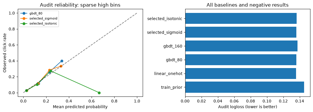
Change one variable: keep the tree fixed, change the probability map
Raw and sigmoid predictions use identical audit rows. Inspect paired logloss differences and a 300-repeat row-bootstrap interval. If it crosses zero, improvement is not established. Row bootstrap does not cover training randomness or user dependence. Isotonic can overfit sparse regions and alter AUC ties.
Predict: which is harder, many missing features or unseen training categories? Inspect segment click rates and sample counts first. This is not a demographic or fairness conclusion.
print(result['paired_sigmoid'])
display(pd.DataFrame([{'segment':s['segment'],'n':s['raw']['n'],'CTR':s['raw']['click_rate'],'raw_logloss':s['raw']['logloss'],'sigmoid_logloss':s['sigmoid']['logloss']} for s in result['segments']]))
failures=result['failures']
print('Eight highest sigmoid-loss audit exposures: clicked count =',sum(r['label'] for r in failures))
print('Detailed failure rows and all per-row predictions stay in the ignored local artifact directory.')
print('Explain: rare positive misses, missingness and unseen categories are hypotheses; anonymous features cannot establish causes.')
Saved notebook output · not executed on this page
{'calibrated_minus_raw_logloss': -6.130390957040765e-05, 'iid_row_bootstrap_95': [-0.00016953362229380587, 6.253575759107997e-05], 'replicates': 300, 'limitation': 'conditional on fitted models; repeated/related rows and one shard limit independence and generalization'}
| segment | n | CTR | raw_logloss | sigmoid_logloss | |
|---|---|---|---|---|---|
| 0 | low_numeric_missing | 17016 | 0.036495 | 0.147043 | 0.146935 |
| 1 | high_numeric_missing | 12912 | 0.028733 | 0.121515 | 0.121515 |
| 2 | any_unseen_category | 11668 | 0.035996 | 0.146929 | 0.146712 |
| 3 | all_categories_seen | 18260 | 0.031325 | 0.129065 | 0.129103 |
Eight highest sigmoid-loss audit exposures: clicked count = 8
Detailed failure rows and all per-row predictions stay in the ignored local artifact directory.
Explain: rare positive misses, missingness and unseen categories are hypotheses; anonymous features cannot establish causes.
Change one variable: bid multiplier in the same simulated market
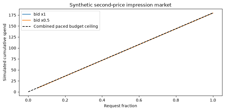
This is not a Criteo replay. Three fictional advertisers face 6,000 requests. True click probabilities, noisy estimates, and all potential clicks are independently generated; traffic is more valuable in the second half. Bids are currency per impression, scored as estimated CTR × fictional click value. The winner pays the second-highest bid including external competition. Each advertiser has budget 60.
Predict first: with seed, budget, and pacing fixed, does changing the multiplier from 1 to 0.5 merely reduce spending, or change which impressions are won? Explain cumulative spend. The later-traffic advantage is a constructed assumption, not grounds for a production bidding policy.
from reclab.auction import market, simulate
synthetic=market(seed=42)
controls=[('bid x1',simulate(synthetic,multiplier=1.,paced=True)),('bid x0.5',simulate(synthetic,multiplier=.5,paced=True))]
display(pd.DataFrame([{'policy':name,**{k:r[k] for k in ['spend','expected_click_value','expected_advertiser_surplus','clicks','budget_ok']}} for name,r in controls]))
fig,ax=plt.subplots(figsize=(8,4))
for name,r in controls:
    ax.plot([t['fraction'] for t in r['trace']],[sum(t['spend']) for t in r['trace']],label=name)
    assert r['budget_ok']
    assert all(max(t['spend'])<=60*t['fraction']+1e-8 for t in r['trace'])
ax.plot([0,1],[0,180],'k--',label='Combined paced budget ceiling')
ax.set(xlabel='Request fraction',ylabel='Simulated cumulative spend',title='Synthetic second-price impression market')
ax.legend();fig.tight_layout();fig.savefig(preview/'18_market.png',dpi=140);plt.show()
print('All fixed-seed policies:')
display(pd.DataFrame([{'policy':r['name'],'seed':r['seed'],'simulated_revenue':r['spend'],'expected_value':r['expected_click_value'],'budget_ok':r['budget_ok']} for r in result['simulations']]))
Saved notebook output · not executed on this page
| policy | spend | expected_click_value | expected_advertiser_surplus | clicks | budget_ok | |
|---|---|---|---|---|---|---|
| 0 | bid x1 | 179.352946 | 363.687988 | 184.335042 | 181 | True |
| 1 | bid x0.5 | 179.667495 | 594.607116 | 414.939622 | 297 | True |
<Figure size 800x400 with 1 Axes>
All fixed-seed policies:
| policy | seed | simulated_revenue | expected_value | budget_ok | |
|---|---|---|---|---|---|
| 0 | flat | 41 | 179.946768 | 310.260151 | True |
| 1 | value | 41 | 179.954436 | 312.713379 | True |
| 2 | value_paced | 41 | 179.523495 | 362.738625 | True |
| 3 | value_paced_halfbid | 41 | 179.584778 | 588.807349 | True |
| 4 | flat | 42 | 179.958459 | 320.400544 | True |
| 5 | value | 42 | 179.950958 | 325.099130 | True |
| 6 | value_paced | 42 | 179.352946 | 363.687988 | True |
| 7 | value_paced_halfbid | 42 | 179.667495 | 594.607116 | True |
| 8 | flat | 43 | 179.880956 | 302.367394 | True |
| 9 | value | 43 | 179.955613 | 328.793557 | True |
| 10 | value_paced | 43 | 179.534714 | 362.467222 | True |
| 11 | value_paced_halfbid | 43 | 179.659235 | 589.567131 | True |
Explain and return to the shared system
In the saved run, the linear model beats both small tree models; sigmoid's small improvement is uncertain, and isotonic does not win. Low ECE for a constant prior does not replace discrimination or proper scoring rules. Simulated pacing and half-price bids explain allocation only in the assumed market. Simultaneous internal bid changes, fixed external competition, and increasing request value limit conclusions.
The workbench calls the trained model on editable anonymous features and independently adjusts simulated budgets. Train explicitly with python -m reclab.ads --download; every run creates a new record and preserves old models. Sources and limits are in docs/ADS_EXPERIMENTS.md. Full Criteo training, online calibration, counterfactual revenue evaluation, and full paper reproduction are not completed here.