18 · 同一系统:真实点击概率与模拟广告决策
先预测 → 只改一个变量 → 执行 → 解释。沿用同一实验记录、下载校验器、FastAPI和工作台07。
真实部分是 Criteo 官方曝光点击日志;模拟部分是单独生成的二价市场。两者没有真实收益或因果联系。日志正负抽样比例未知,模型概率只属于公开样本分布。
先预测:更复杂的树模型一定超过线性模型吗?校准一定改善 logloss 吗?恒定先验的 ECE 很小就代表有用吗?
from pathlib import Path
import sys
ROOT=Path.cwd()
if not (ROOT/'reclab').is_dir(): ROOT=ROOT.parent
sys.path.insert(0,str(ROOT))
import numpy as np
import pandas as pd
import matplotlib.pyplot as plt
from reclab.ads import latest
from reclab.paths import ARTIFACTS
receipt, result=latest()
folder=ARTIFACTS/'experiments/ads'/receipt['run_id']
print('Shared run:', receipt['run_id'])
print(result['scope'])
display(pd.DataFrame(result['splits']).T)
assert sum(x['n'] for x in result['splits'].values())==receipt['config']['rows']
print('Feature duplicate rows:',result['feature_duplicate_rows'])
print('Grouping uses features only; no temporal/user holdout is claimed.')
Notebook 保存的输出 · 本页未执行
Shared run: 20261030T125738-f82b6582
Criteo official sampled click logs: first 200,000 rows of one 766,864-row parquet shard (2015-02-15). Real CTR task on a subsampled distribution. Auction is a separate synthetic market.
| n | positives | click_rate | unique_feature_groups | |
|---|---|---|---|---|
| train | 109935.0 | 3614.0 | 0.032874 | 109934.0 |
| select | 29984.0 | 1016.0 | 0.033885 | 29984.0 |
| calibration | 30153.0 | 1023.0 | 0.033927 | 30153.0 |
| audit | 29928.0 | 992.0 | 0.033146 | 29928.0 |
Feature duplicate rows: 1
Grouping uses features only; no temporal/user holdout is claimed.
先比较真实概率,而不是套用检索指标
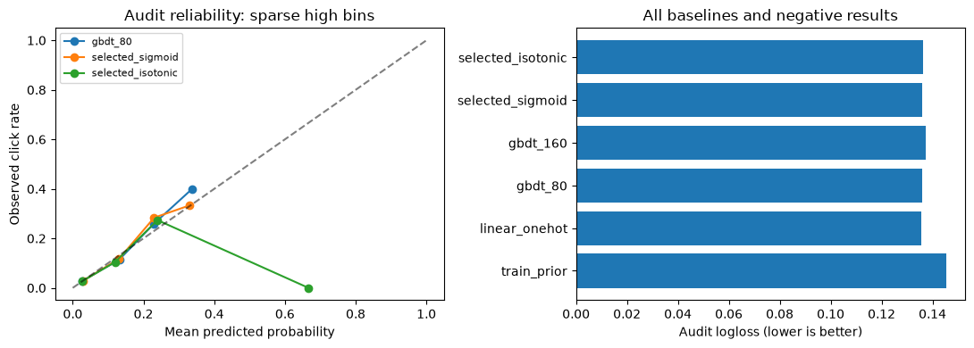
AUC衡量区分度;logloss、Brier衡量概率质量。ECE采用10个等宽箱,低点击率时恒定先验也可得到很小的ECE,不能独立选型。编码器仅拟合train;select仅在80/160棵树之间选择,calibration单独拟合sigmoid和isotonic。审计不选型,线性模型仍是独立对照。
执行下面一格,观察负结果。系数全表在本机实验目录 linear_coefficients.csv,权重不上传。
summary=pd.DataFrame([{'method':r['method'],**{k:r['audit'][k] for k in ['auc','logloss','brier','ece']},'fit_seconds':r['fit_seconds']} for r in result['rows']])
display(summary.round(6))
print('GBDT family selected by select logloss:',result['selected_base'])
fig,axes=plt.subplots(1,2,figsize=(11,4))
for row in result['rows']:
    if row['method'] in [result['selected_base'],'selected_sigmoid','selected_isotonic']:
        bins=row['audit']['reliability']
        axes[0].plot([b['mean_probability'] for b in bins],[b['click_rate'] for b in bins],marker='o',label=row['method'])
axes[0].plot([0,1],[0,1],'k--',alpha=.5)
axes[0].set(xlabel='Mean predicted probability',ylabel='Observed click rate',title='Audit reliability: sparse high bins')
axes[0].legend(fontsize=8)
axes[1].barh(summary.method,summary.logloss)
axes[1].set(xlabel='Audit logloss (lower is better)',title='All baselines and negative results')
fig.tight_layout()
preview=ROOT/'artifacts/notebook-previews';preview.mkdir(parents=True,exist_ok=True)
fig.savefig(preview/'18_probability.png',dpi=140)
plt.show()
Notebook 保存的输出 · 本页未执行
| method | auc | logloss | brier | ece | fit_seconds | |
|---|---|---|---|---|---|---|
| 0 | train_prior | 0.500000 | 0.145515 | 0.032048 | 0.000272 | 0.000000 |
| 1 | linear_onehot | 0.721468 | 0.135423 | 0.031193 | 0.004382 | 4.102396 |
| 2 | gbdt_80 | 0.706329 | 0.136029 | 0.031221 | 0.001738 | 0.555461 |
| 3 | gbdt_160 | 0.703035 | 0.137404 | 0.031358 | 0.005350 | 0.932227 |
| 4 | selected_sigmoid | 0.706329 | 0.135968 | 0.031219 | 0.001149 | 0.008740 |
| 5 | selected_isotonic | 0.703064 | 0.136437 | 0.031302 | 0.001163 | 0.006879 |
GBDT family selected by select logloss: gbdt_80
<Figure size 1100x400 with 2 Axes>
只改一个变量:固定树模型,改变概率映射
原始分数与sigmoid使用完全相同的审计行。查看配对logloss差异及300次行bootstrap区间;区间跨零时,不能说改善已被证实。行bootstrap没有覆盖训练随机性或用户相关性。Isotonic可能在样本稀疏区过拟合并改变AUC的并列关系。
预测:缺失多和出现训练未见类别的样本,哪一段更难?先看各段点击率与样本数;这不是人口属性或公平性结论。
print(result['paired_sigmoid'])
display(pd.DataFrame([{'segment':s['segment'],'n':s['raw']['n'],'CTR':s['raw']['click_rate'],'raw_logloss':s['raw']['logloss'],'sigmoid_logloss':s['sigmoid']['logloss']} for s in result['segments']]))
failures=result['failures']
print('Eight highest sigmoid-loss audit exposures: clicked count =',sum(r['label'] for r in failures))
print('Detailed failure rows and all per-row predictions stay in the ignored local artifact directory.')
print('Explain: rare positive misses, missingness and unseen categories are hypotheses; anonymous features cannot establish causes.')
Notebook 保存的输出 · 本页未执行
{'calibrated_minus_raw_logloss': -6.130390957040765e-05, 'iid_row_bootstrap_95': [-0.00016953362229380587, 6.253575759107997e-05], 'replicates': 300, 'limitation': 'conditional on fitted models; repeated/related rows and one shard limit independence and generalization'}
| segment | n | CTR | raw_logloss | sigmoid_logloss | |
|---|---|---|---|---|---|
| 0 | low_numeric_missing | 17016 | 0.036495 | 0.147043 | 0.146935 |
| 1 | high_numeric_missing | 12912 | 0.028733 | 0.121515 | 0.121515 |
| 2 | any_unseen_category | 11668 | 0.035996 | 0.146929 | 0.146712 |
| 3 | all_categories_seen | 18260 | 0.031325 | 0.129065 | 0.129103 |
Eight highest sigmoid-loss audit exposures: clicked count = 8
Detailed failure rows and all per-row predictions stay in the ignored local artifact directory.
Explain: rare positive misses, missingness and unseen categories are hypotheses; anonymous features cannot establish causes.
只改一个变量:同一模拟市场的出价倍数
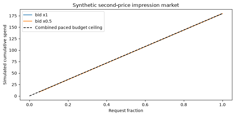
以下不是Criteo回放。3个虚构广告主,6000次请求,独立生成真实点击概率、带噪估计概率和所有潜在点击;后半程流量更有价值。报价单位为“每曝光货币”,得分是估计点击率×虚构点击价值;赢家支付次高报价(含外部竞争价)。每广告主预算60。
先预测:固定seed、预算和pacing,仅将倍数从1降为0.5,会少花钱还是赢得不同曝光?再解释累计花费曲线。合成市场中的后半程优势是构造假设,不能据此发布生产出价策略。
from reclab.auction import market, simulate
synthetic=market(seed=42)
controls=[('bid x1',simulate(synthetic,multiplier=1.,paced=True)),('bid x0.5',simulate(synthetic,multiplier=.5,paced=True))]
display(pd.DataFrame([{'policy':name,**{k:r[k] for k in ['spend','expected_click_value','expected_advertiser_surplus','clicks','budget_ok']}} for name,r in controls]))
fig,ax=plt.subplots(figsize=(8,4))
for name,r in controls:
    ax.plot([t['fraction'] for t in r['trace']],[sum(t['spend']) for t in r['trace']],label=name)
    assert r['budget_ok']
    assert all(max(t['spend'])<=60*t['fraction']+1e-8 for t in r['trace'])
ax.plot([0,1],[0,180],'k--',label='Combined paced budget ceiling')
ax.set(xlabel='Request fraction',ylabel='Simulated cumulative spend',title='Synthetic second-price impression market')
ax.legend();fig.tight_layout();fig.savefig(preview/'18_market.png',dpi=140);plt.show()
print('All fixed-seed policies:')
display(pd.DataFrame([{'policy':r['name'],'seed':r['seed'],'simulated_revenue':r['spend'],'expected_value':r['expected_click_value'],'budget_ok':r['budget_ok']} for r in result['simulations']]))
Notebook 保存的输出 · 本页未执行
| policy | spend | expected_click_value | expected_advertiser_surplus | clicks | budget_ok | |
|---|---|---|---|---|---|---|
| 0 | bid x1 | 179.352946 | 363.687988 | 184.335042 | 181 | True |
| 1 | bid x0.5 | 179.667495 | 594.607116 | 414.939622 | 297 | True |
<Figure size 800x400 with 1 Axes>
All fixed-seed policies:
| policy | seed | simulated_revenue | expected_value | budget_ok | |
|---|---|---|---|---|---|
| 0 | flat | 41 | 179.946768 | 310.260151 | True |
| 1 | value | 41 | 179.954436 | 312.713379 | True |
| 2 | value_paced | 41 | 179.523495 | 362.738625 | True |
| 3 | value_paced_halfbid | 41 | 179.584778 | 588.807349 | True |
| 4 | flat | 42 | 179.958459 | 320.400544 | True |
| 5 | value | 42 | 179.950958 | 325.099130 | True |
| 6 | value_paced | 42 | 179.352946 | 363.687988 | True |
| 7 | value_paced_halfbid | 42 | 179.667495 | 594.607116 | True |
| 8 | flat | 43 | 179.880956 | 302.367394 | True |
| 9 | value | 43 | 179.955613 | 328.793557 | True |
| 10 | value_paced | 43 | 179.534714 | 362.467222 | True |
| 11 | value_paced_halfbid | 43 | 179.659235 | 589.567131 | True |
解释并回到共享系统
本轮线性模型胜过两个小树模型;sigmoid的小幅改善不确定,isotonic没有胜出。恒定先验的低ECE不能替代区分度和适当评分。模拟pacing和半价出价只说明预设市场中的资源分配,所有广告主同时改变报价、外部竞价不变、请求价值随时间增长等假设限制结论。
工作台07可修改匿名特征并实际调用训练模型,也可独立调整模拟市场预算。训练需显式执行 python -m reclab.ads --download,每次创建新记录,不覆盖旧模型。详细来源与边界见 docs/ADS_EXPERIMENTS.md。没有完成全量Criteo、线上校准、反事实收益评估或论文完整复现。