01 · Real data, features, and ItemCF
Goal
Follow a recommendation through real Python code: data files → causal history → user features → ItemCF scores → filtering previously seen items.
By default, this notebook only reads existing data and baselines. It does not download again, alter the original stream-processing lab, or update models. Use Shift+Enter one cell at a time; open and edit reclab/*.py in the file browser.
English companion. All instructional Markdown is translated. Experiment code, Chinese language examples, execution counts, and saved outputs remain as in the source edition; historical output text may therefore be Chinese. The initial setup cell anchors the working directory and Python import path for this companion's deeper folder; it does not change the experiment. Saved outputs are historical evidence, not a new run. Run from the top after preparing the required data and models.
# English companions live one directory deeper; keep the original experiment code unchanged.
from pathlib import Path as _TranslationPath
import os as _translation_os
import sys as _translation_sys
_translation_root = next((p for p in [_TranslationPath.cwd(), *_TranslationPath.cwd().parents]
                          if (p / "reclab").is_dir()), None)
if _translation_root is None:
    raise RuntimeError("Open this notebook from inside the Search Recommendation Ads Lab checkout.")
_translation_os.chdir(_translation_root)
if str(_translation_root) not in _translation_sys.path:
    _translation_sys.path.insert(0, str(_translation_root))
Setup
Select the project's Search Recommendation Ads Lab (Python 3.12) kernel (older saved metadata may call it Recommendation Lab). Inputs are data/processed/events.parquet, manifest.json, and artifacts/baselines/. The dataset is Retailrocket.
The task is retrieval of new user–item interactions for warm items after the training cutoff. A view is a behavior, not a recommendation impression; no interaction does not mean an unclicked impression.
from pathlib import Path
import sys
import inspect
import numpy as np
import pandas as pd
import matplotlib.pyplot as plt
from IPython.display import display, Code


PROJECT = next(p for p in [Path.cwd(), *Path.cwd().parents]
               if (p / "reclab/models.py").exists())
if str(PROJECT) not in sys.path:
    sys.path.insert(0, str(PROJECT))
from reclab.data import Dataset
from reclab.paths import ARTIFACTS, PROCESSED, read_json


plt.rcParams.update({"figure.figsize": (9, 3.8), "font.size": 11,
    "axes.spines.top": False, "axes.spines.right": False,
    "axes.labelcolor": "#182b2b", "text.color": "#182b2b",
    "axes.facecolor": "white", "figure.facecolor": "white",
    "grid.color": "#d4ddda", "axes.axisbelow": True})
dataset = Dataset()
print("Project:", PROJECT)
print("Dataset version:", dataset.manifest["dataset_version"])
print("Python:", sys.executable)
assert Path(sys.executable).parent == PROJECT / ".venv/bin", "请选择 Recommendation Lab 内核"
Saved notebook output · not executed on this page
Project: /Users/lizuolin/local/recommendation-lab
Dataset version: 2772cab0aca8cb81
Python: /Users/lizuolin/local/recommendation-lab/.venv/bin/python
Steps
1. Inspect files and actual time boundaries
These numbers come from the frozen manifest, the same data used by the workbench.
m = dataset.manifest
display(pd.Series({k: m[k] for k in ["raw_events", "cohort_users", "catalog_items", "cohort_events", "feature_version"]}, name="value").to_frame())
boundaries = pd.Series({"start": m["start_ms"], "train_end": m["train_end_ms"], "valid_end": m["valid_end_ms"], "end": m["end_ms"]})
display(pd.to_datetime(boundaries, unit="ms", utc=True).to_frame("UTC boundary"))
display(dataset.events.head(5))
Saved notebook output · not executed on this page
| value | |
|---|---|
| raw_events | 2756101 |
| cohort_users | 6734 |
| catalog_items | 5000 |
| cohort_events | 265884 |
| feature_version | history-id-v1 |
| UTC boundary | |
|---|---|
| start | 2015-05-03 03:00:04.384000+00:00 |
| train_end | 2015-08-07 17:23:52.766000+00:00 |
| valid_end | 2015-08-28 10:11:50.277000+00:00 |
| end | 2015-09-18 02:59:47.788000+00:00 |
| timestamp | visitorid | event | itemid | transactionid | split | item_idx | user_idx | weight | event_id | |
|---|---|---|---|---|---|---|---|---|---|---|
| 0 | 1430622124584 | 1346730 | view | 252280 | NaN | train | 0 | 6434 | 1.0 | 40 |
| 1 | 1430622325414 | 1222911 | view | 278143 | NaN | train | 0 | 5847 | 1.0 | 87 |
| 2 | 1430622876445 | 1359701 | view | 173766 | NaN | train | 0 | 6498 | 1.0 | 219 |
| 3 | 1430623120795 | 122517 | view | 75694 | NaN | train | 0 | 529 | 1.0 | 295 |
| 4 | 1430623150639 | 122517 | view | 443197 | NaN | train | 0 | 529 | 1.0 | 305 |
2. Query Parquet with SQL
DuckDB queries in memory; no container is started. item_idx=0 denotes an item outside the training vocabulary.
import duckdb
with duckdb.connect(":memory:") as con:
    split_summary = con.execute("""
        SELECT split, count(*) AS events,
               count(DISTINCT visitorid) AS users,
               count(*) FILTER (WHERE item_idx = 0) AS oov_events
        FROM read_parquet(?) GROUP BY split ORDER BY split
    """, [str(PROCESSED / "events.parquet")]).df()
display(split_summary)
Saved notebook output · not executed on this page
| split | events | users | oov_events | |
|---|---|---|---|---|
| 0 | test | 10350 | 472 | 7692 |
| 1 | train | 240095 | 6734 | 119080 |
| 2 | valid | 15439 | 617 | 10859 |
3. Choose a user and inspect the actual model history
After changing USER_POSITION or HISTORY_WINDOW, rerun the following cells. Category is explanatory metadata; the current two-tower model does not use it as an input.
USER_POSITION = 0
HISTORY_WINDOW = 20
TOP_K = 10
eligible, audit = dataset.evaluation("valid", 1000)
user_idx = list(eligible)[USER_POSITION]
history = dataset.histories[user_idx]
user_events = dataset.train[dataset.train.user_idx == user_idx].sort_values("timestamp", kind="stable")
print("User ID:", dataset.users[user_idx], "User index:", user_idx)
print("Training-only history:", history[-HISTORY_WINDOW:])
preview = user_events.tail(HISTORY_WINDOW)[["timestamp", "event", "itemid", "item_idx"]].copy()
preview["timestamp"] = pd.to_datetime(preview.timestamp, unit="ms", utc=True)
display(preview)
assert user_events.timestamp.max() < m["train_end_ms"]
Saved notebook output · not executed on this page
User ID: 1055524 User index: 5071
Training-only history: [4008, 2088, 2633, 3949, 211, 211, 2913]
| timestamp | event | itemid | item_idx | |
|---|---|---|---|---|
| 51317 | 2015-05-23 13:54:45.097000+00:00 | view | 374092 | 4008 |
| 51319 | 2015-05-23 13:56:22.761000+00:00 | view | 200231 | 2088 |
| 51320 | 2015-05-23 13:57:32.977000+00:00 | view | 248327 | 2633 |
| 51321 | 2015-05-23 13:58:58.224000+00:00 | view | 367664 | 3949 |
| 52462 | 2015-05-23 23:38:32.172000+00:00 | view | 21253 | 211 |
| 52472 | 2015-05-23 23:40:07.466000+00:00 | addtocart | 21253 | 211 |
| 209735 | 2015-07-23 21:57:59.118000+00:00 | view | 272770 | 2913 |
4. Trace a real sample back to its history
The positive target is a newly interacted-with item, and every history event must strictly precede it. Read the function source, then inspect an actual sample.
display(Code(inspect.getsource(Dataset.examples), language="python"))
sample_users, sample_history, sample_targets, sample_times = dataset.examples(HISTORY_WINDOW)
selected = np.flatnonzero(sample_users == user_idx)
assert len(selected), "当前用户没有可用训练样本,请换 USER_POSITION"
j = int(selected[0])
context = sample_history[j][sample_history[j] != 0].tolist()
target = int(sample_targets[j])
prior = user_events[user_events.timestamp < sample_times[j]]
display(pd.DataFrame([{"user_idx": user_idx, "history": context,
    "target_item_idx": target, "target_time_utc": pd.to_datetime(sample_times[j], unit="ms", utc=True)}]))
assert context == prior.item_idx.astype(int).tail(HISTORY_WINDOW).tolist()
assert target not in set(prior.item_idx)
Saved notebook output · not executed on this page
    def examples(self, history_len=20):
        users, histories, targets, times = [], [], [], []
        for user, group in self.train.groupby("user_idx", sort=True):
            past, seen, last_time = [], set(), -1
            for row in group.sort_values("timestamp", kind="stable").itertuples():
                item = int(row.item_idx)
                if (
                    len(seen) >= 2
                    and item not in seen
                    and last_time < int(row.timestamp)
                ):
                    h = past[-history_len:]
                    users.append(int(user))
                    histories.append([0] * (history_len - len(h)) + h)
                    targets.append(item)
                    times.append(int(row.timestamp))
                past.append(item)
                seen.add(item)
                last_time = int(row.timestamp)
        return (
            np.array(users, dtype=np.int64),
            np.array(histories, dtype=np.int64),
            np.array(targets, dtype=np.int64),
            np.array(times, dtype=np.int64),
)| user_idx | history | target_item_idx | target_time_utc | |
|---|---|---|---|---|
| 0 | 5071 | [4008, 2088] | 2633 | 2015-05-23 13:57:32.977000+00:00 |
5. Read ItemCF source and compute recommendations
This uses the saved neighbor matrix. The current variant penalizes highly active users and retains the top 100 neighbors per item. Scoring applies decaying weights to the last 50 interactions.
from scipy import sparse
from reclab.retrieval import itemcf, cf_scores, topk
display(Code(inspect.getsource(itemcf), language="python"))
similarity = sparse.load_npz(ARTIFACTS / "baselines/itemcf.npz")
scores = cf_scores(similarity, history, dataset.n_items)
recommendations = topk(scores, TOP_K, dataset.seen[user_idx])
display(pd.DataFrame([{**dataset.items[i-1], "itemcf_score": float(scores[i])}
                      for i in recommendations]))
assert not set(recommendations) & dataset.seen[user_idx]
Saved notebook output · not executed on this page
def itemcf(dataset):
    pairs = dataset.train[["user_idx", "item_idx"]].drop_duplicates()
    matrix = sparse.csr_matrix(
        (np.ones(len(pairs), dtype=np.float32), (pairs.user_idx, pairs.item_idx)),
        shape=(dataset.n_users, dataset.n_items),
    )
    # Inverse user activity reduces extremely active users' co-occurrence contribution.
    activity = np.asarray(matrix.sum(1)).ravel()
    weighted = sparse.diags(1 / np.log1p(np.maximum(activity, 1))) @ matrix
    co = (matrix.T @ weighted).tocsr()
    frequency = np.asarray(matrix.sum(0)).ravel()
    norm = sparse.diags(1 / np.sqrt(np.maximum(frequency, 1)))
    sim = (norm @ co @ norm).tocsr()
    sim.setdiag(0)
    sim.eliminate_zeros()
    # Keep 100 neighbors per item, bounded memory and easy inspection.
    for i in range(sim.shape[0]):
        a, b = sim.indptr[i : i + 2]
        if b - a > 100:
            loc = np.argpartition(sim.data[a:b], -100)[:-100]
            sim.data[a + loc] = 0
    sim.eliminate_zeros()
return sim| item_idx | item_id | category | category_asof_ms | train_events | itemcf_score | |
|---|---|---|---|---|---|---|
| 0 | 3720 | 348157 | 1666 | 1433646000000 | 101 | 0.145335 |
| 1 | 2727 | 257040 | 683 | 1433041200000 | 1324 | 0.138386 |
| 2 | 991 | 94296 | 1565 | 1431226800000 | 90 | 0.112878 |
| 3 | 4051 | 378045 | 1666 | 1435460400000 | 224 | 0.111876 |
| 4 | 722 | 69974 | 818 | 1433041200000 | 249 | 0.109628 |
| 5 | 3794 | 354733 | 23 | 1431226800000 | 82 | 0.108164 |
| 6 | 3402 | 317899 | 1666 | 1431226800000 | 87 | 0.103384 |
| 7 | 4619 | 432152 | 683 | 1431226800000 | 382 | 0.101446 |
| 8 | 3596 | 337512 | 316 | 1431226800000 | 83 | 0.099587 |
| 9 | 4101 | 382751 | 683 | 1435460400000 | 460 | 0.099382 |
6. How is one score accumulated?
Expand the contribution of every history item for the first candidate, then verify their sum.
chosen_item = recommendations[0]
recent = history[-50:]
recency_weights = np.geomspace(0.2, 1.0, len(recent))
contributions = pd.DataFrame([{"history_item_idx": i,
    "history_item_id": dataset.items[i-1]["item_id"],
    "similarity": float(similarity[i, chosen_item]), "weight": float(w),
    "contribution": float(similarity[i, chosen_item]) * w}
    for i, w in zip(recent, recency_weights)])
display(contributions.sort_values("contribution", ascending=False).head(10))
print("Sum of contributions:", contributions.contribution.sum())
print("Saved scorer output:", float(scores[chosen_item]))
assert np.isclose(contributions.contribution.sum(), scores[chosen_item], atol=1e-6)
Saved notebook output · not executed on this page
| history_item_idx | history_item_id | similarity | weight | contribution | |
|---|---|---|---|---|---|
| 5 | 211 | 21253 | 0.100419 | 0.764724 | 0.076793 |
| 4 | 211 | 21253 | 0.100419 | 0.584804 | 0.058725 |
| 2 | 2633 | 248327 | 0.028706 | 0.341995 | 0.009817 |
| 0 | 4008 | 374092 | 0.000000 | 0.200000 | 0.000000 |
| 1 | 2088 | 200231 | 0.000000 | 0.261532 | 0.000000 |
| 3 | 3949 | 367664 | 0.000000 | 0.447214 | 0.000000 |
| 6 | 2913 | 272770 | 0.000000 | 1.000000 | 0.000000 |
Sum of contributions: 0.14533540791386457
Saved scorer output: 0.14533540606498718
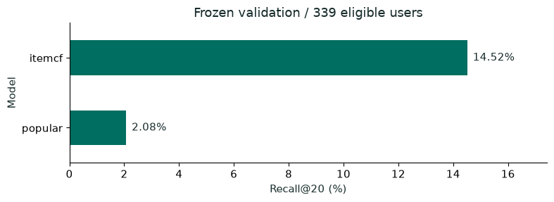
7. Compare existing baseline results
The validation window, full training vocabulary, and training-history seen-item filter are identical. Scores cover only the currently evaluable active, warm-start users.
baseline = read_json(ARTIFACTS / "baselines/metrics.json")
result = pd.DataFrame([{"model": name, "Recall@20": row["metrics"]["recall@20"],
    "NDCG@20": row["metrics"]["ndcg@20"], "users": row["audit"]["evaluated_users"]}
    for name, row in baseline["models"].items()]).set_index("model")
display(result)
ax = (result["Recall@20"] * 100).plot.barh(color="#006e60", figsize=(8, 3))
ax.set(xlabel="Recall@20 (%)", ylabel="Model",
       title=f"Frozen validation / {int(result.users.iloc[0])} eligible users")
ax.set_xlim(left=0)
for y, value in enumerate(result["Recall@20"] * 100):
    ax.text(value + 0.2, y, f"{value:.2f}%", va="center")
ax.set_xlim(0, max(result["Recall@20"] * 100) * 1.2)
plt.tight_layout(); plt.show()
Saved notebook output · not executed on this page
| Recall@20 | NDCG@20 | users | |
|---|---|---|---|
| model | |||
| popular | 0.020754 | 0.017910 | 339 |
| itemcf | 0.145167 | 0.079874 | 339 |
<Figure size 800x300 with 1 Axes>
Checks
The assertions check time boundaries, causal samples, seen-item filtering, and individual ItemCF score contributions. Tables retain the original precise values.
Next steps
Predict first: if history is truncated to the last three items, which candidates should change? Use cf_scores(similarity, history[-3:], ...) as a single-user counterfactual comparison; it is not an offline metric from a retrained model.
Open 02_TwoTower_HandsOn.ipynb next. Related lecture topics: ItemCF, categorical features, and two-tower training samples.