16 · Deeper recommendation experiments: negatives, sequences, and indexes
Predict first: are hard negatives always better? Must a sequence model beat mean pooling? Does a faster index mean more accurate recommendations?
Reuse the original Retailrocket time split, causal samples, full-catalog validation metrics, and workbench. Read only the latest completed recommendation experiment; no automatic retraining. Train explicitly with python -m reclab.deep_recommendation. The budget is 12,000 samples × four epochs × two seeds. Models are not trained to convergence, so this does not establish architectural limits. The reserved test window is not used.
English companion. All instructional Markdown is translated. Experiment code, Chinese language examples, execution counts, and saved outputs remain as in the source edition; historical output text may therefore be Chinese. The initial setup cell anchors the working directory and Python import path for this companion's deeper folder; it does not change the experiment. Saved outputs are historical evidence, not a new run. Run from the top after preparing the required data and models.
# English companions live one directory deeper; keep the original experiment code unchanged.
from pathlib import Path as _TranslationPath
import os as _translation_os
import sys as _translation_sys
_translation_root = next((p for p in [_TranslationPath.cwd(), *_TranslationPath.cwd().parents]
                          if (p / "reclab").is_dir()), None)
if _translation_root is None:
    raise RuntimeError("Open this notebook from inside the Search Recommendation Ads Lab checkout.")
_translation_os.chdir(_translation_root)
if str(_translation_root) not in _translation_sys.path:
    _translation_sys.path.insert(0, str(_translation_root))
from pathlib import Path
import sys, json
ROOT = Path.cwd()
if not (ROOT/'reclab').is_dir(): ROOT = ROOT.parent
sys.path.insert(0,str(ROOT))
import pandas as pd
import matplotlib.pyplot as plt
from reclab.experiments import catalog, result
runs=[r for r in catalog() if r['domain']=='recommendation' and r['state']=='completed' and not r.get('annotation',{}).get('superseded')]
assert runs, '先运行 python -m reclab.deep_recommendation'
receipt=runs[-1]; experiment=result('recommendation',receipt['run_id'])
print(receipt['run_id'], 'samples',experiment['samples'], 'users',experiment['evaluation_users'])
print(experiment['scope'])
frame=pd.DataFrame([{k:v for k,v in row.items() if k not in ('loss','index','shuffled')} for row in experiment['rows']])
display(frame[['encoder','sampler','seed','parameters','ndcg@20','recall@20','coverage@20']])
Saved notebook output · not executed on this page
20261030T123443-578def14 samples 12000 users 339
Bounded real-data ablation; loss is not CTR; popularity proposal uses train-only aggregate frequency; hard negatives are model-selected from 16 unseen-prefix candidates. Validation is a visible development benchmark, not an untouched audit.
| encoder | sampler | seed | parameters | ndcg@20 | recall@20 | coverage@20 | |
|---|---|---|---|---|---|---|---|
| 0 | mean | uniform | 42 | 120624 | 0.007160 | 0.007526 | 0.3510 |
| 1 | mean | popular | 42 | 120624 | 0.003932 | 0.005230 | 0.4450 |
| 2 | mean | hard | 42 | 120624 | 0.005239 | 0.008450 | 0.2938 |
| 3 | gru | uniform | 42 | 124224 | 0.002641 | 0.003189 | 0.2300 |
| 4 | attention | uniform | 42 | 123504 | 0.004672 | 0.007186 | 0.1514 |
| 5 | mean | uniform | 2026 | 120624 | 0.001771 | 0.002463 | 0.3554 |
| 6 | mean | popular | 2026 | 120624 | 0.002815 | 0.005158 | 0.4232 |
| 7 | mean | hard | 2026 | 120624 | 0.001483 | 0.002045 | 0.2626 |
| 8 | gru | uniform | 2026 | 124224 | 0.002450 | 0.002017 | 0.2586 |
| 9 | attention | uniform | 2026 | 123504 | 0.003738 | 0.002698 | 0.1406 |
1 · Negative sampling: change only the proposal distribution first
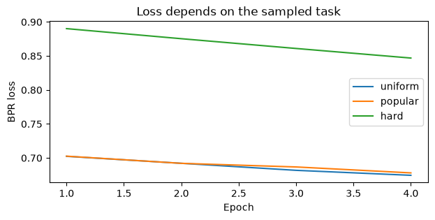
For the same mean encoder, compare uniform sampling, training frequency^.75, and the highest-scoring hard negative among 16 candidates. Mask the current positive and causal prefix; unknown future positives may be false negatives. All arms share samples, batch order, initialization seeds, and optimization budget. Losses across different negative distributions are not directly comparable.
means=frame[frame.encoder=='mean'].groupby('sampler')[['ndcg@20','recall@20','coverage@20']].agg(['mean','std'])
display(means)
fig,ax=plt.subplots(figsize=(7,3))
for row in experiment['rows']:
    if row['encoder']=='mean' and row['seed']==42: ax.plot(range(1,len(row['loss'])+1),row['loss'],label=row['sampler'])
ax.set(xlabel='Epoch',ylabel='BPR loss',title='Loss depends on the sampled task');ax.legend();plt.show()
Saved notebook output · not executed on this page
| ndcg@20 | recall@20 | coverage@20 | ||||
|---|---|---|---|---|---|---|
| mean | std | mean | std | mean | std | |
| sampler | ||||||
| hard | 0.003361 | 0.002656 | 0.005247 | 0.004528 | 0.2782 | 0.022062 |
| popular | 0.003374 | 0.000790 | 0.005194 | 0.000051 | 0.4341 | 0.015415 |
| uniform | 0.004466 | 0.003811 | 0.004994 | 0.003580 | 0.3532 | 0.003111 |
<Figure size 700x300 with 1 Axes>
2 · Sequences: inspect both parameter count and order
Compare mean pooling, GRU, and self-attention pooling with positional encodings. These are teaching sequence encoders, not full SASRec or DIN reproductions. GRU packs left-padded sequences; attention masks padding. The models have no user-ID feature.
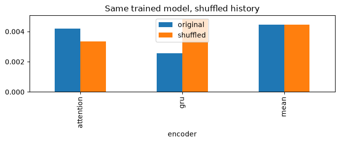
Shuffle histories at inference for a within-model ablation. This measures sensitivity to order, not causal gains from order. Two seeds are also insufficient to claim statistical significance.
uniform=frame[frame.sampler=='uniform']
display(uniform.groupby('encoder')[['ndcg@20','recall@20','parameters']].mean())
shuffle=pd.DataFrame([{'encoder':r['encoder'],'seed':r['seed'],'original':r['ndcg@20'],'shuffled':r['shuffled']['ndcg@20']} for r in experiment['rows'] if r['sampler']=='uniform'])
display(shuffle)
shuffle.groupby('encoder')[['original','shuffled']].mean().plot.bar(figsize=(7,3),title='Same trained model, shuffled history');plt.tight_layout();plt.show()
Saved notebook output · not executed on this page
| ndcg@20 | recall@20 | parameters | |
|---|---|---|---|
| encoder | |||
| attention | 0.004205 | 0.004942 | 123504.0 |
| gru | 0.002546 | 0.002603 | 124224.0 |
| mean | 0.004466 | 0.004994 | 120624.0 |
| encoder | seed | original | shuffled | |
|---|---|---|---|---|
| 0 | mean | 42 | 0.007160 | 0.007160 |
| 1 | gru | 42 | 0.002641 | 0.006853 |
| 2 | attention | 42 | 0.004672 | 0.003519 |
| 3 | mean | 2026 | 0.001771 | 0.001771 |
| 4 | gru | 2026 | 0.002450 | 0.002790 |
| 5 | attention | 2026 | 0.003738 | 0.003169 |
<Figure size 700x300 with 1 Axes>
3 · Indexes: separate recommendation recall from retrieval approximation
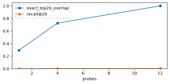
Reuse the course's 12-cluster coarse index with probes=1/4/12. Record scan volume, overlap with exact top 20, and Recall/NDCG against real labels. Scanning all 12 clusters should reduce to exact retrieval. Do not assume approximation is faster on a small vocabulary.
index=pd.DataFrame([{'seed':r['seed'],**i} for r in experiment['rows'] for i in r.get('index',[])])
assert (index[index.probes==12].exact_top20_overlap==1).all()
display(index)
index.groupby('probes')[['exact_top20_overlap','recall@20']].mean().plot(marker='o',figsize=(7,3));plt.ylim(0,1.05);plt.show()
Saved notebook output · not executed on this page
| seed | probes | exact_top20_overlap | mean_scanned | seconds | recall@20 | ndcg@20 | mrr@20 | hit_rate@20 | |
|---|---|---|---|---|---|---|---|---|---|
| 0 | 42 | 1 | 0.287463 | 421.404130 | 0.034856 | 0.002371 | 0.002808 | 0.005616 | 0.026549 |
| 1 | 42 | 4 | 0.708997 | 1673.713864 | 0.079289 | 0.006380 | 0.007160 | 0.012372 | 0.032448 |
| 2 | 42 | 12 | 1.000000 | 5000.000000 | 0.185076 | 0.007526 | 0.007160 | 0.010735 | 0.035398 |
| 3 | 2026 | 1 | 0.301622 | 407.519174 | 0.034720 | 0.002246 | 0.002125 | 0.004994 | 0.026549 |
| 4 | 2026 | 4 | 0.743215 | 1643.324484 | 0.078714 | 0.001008 | 0.001674 | 0.005415 | 0.020649 |
| 5 | 2026 | 12 | 1.000000 | 5000.000000 | 0.194151 | 0.002463 | 0.001771 | 0.003196 | 0.020649 |
<Figure size 700x300 with 1 Axes>
4 · Change one variable yourself
Record a prediction, change one of history, dim, epochs, or samples in Config, run a new experiment, and rerun this chapter. Each experiment creates a new directory and preserves old weights. Compare budget, parameter count, popularity bias, and coverage alongside quality. The original formal two-tower models and competition workflow remain independently usable.
from reclab.deep_recommendation import Config, SequenceEncoder, negatives
import inspect
print(inspect.getsource(negatives))
assert len(experiment['rows'])==len(receipt['config']['seeds'])*5
assert all(len(r['loss'])==receipt['config']['epochs'] for r in experiment['rows'])
print('PASS: complete controls and index parity checked')
Saved notebook output · not executed on this page
def negatives(history, positives, probability, rng, width=1):
    # Only causal prefix and current target are excluded. Unknown future positives remain unknown.
    out = rng.choice(len(probability), size=(len(history), width), p=probability)
    blocked = [set(row) | {int(pos), 0} for row, pos in zip(history, positives)]
    if any(sum(probability[i] for i in b) >= 1 - 1e-12 for b in blocked):
        raise ValueError('No negative support')
    for row, excluded in enumerate(blocked):
        for _ in range(100):
            bad = np.isin(out[row], list(excluded))
            if not bad.any():
                break
            out[row, bad] = rng.choice(len(probability), size=int(bad.sum()), p=probability)
        else:
            raise RuntimeError('Negative sampling failed')
    return out

PASS: complete controls and index parity checked