16 · 深入推荐:负例、序列与索引
先预测:难负例一定更好?顺序模型一定胜过均值?索引更快是否意味着推荐更准?
本章复用原Retailrocket时间切分、因果样本、全库验证指标及工作台。只读取最新完成的推荐实验,不自动重训。训练命令:python -m reclab.deep_recommendation。训练预算12000样本×4轮×2种子;未训练至收敛,不代表结构上限。没有使用保留测试窗口。
PYTHON · 01
from pathlib import Path
import sys, json
ROOT = Path.cwd()
if not (ROOT/'reclab').is_dir(): ROOT = ROOT.parent
sys.path.insert(0,str(ROOT))
import pandas as pd
import matplotlib.pyplot as plt
from reclab.experiments import catalog, result
runs=[r for r in catalog() if r['domain']=='recommendation' and r['state']=='completed' and not r.get('annotation',{}).get('superseded')]
assert runs, '先运行 python -m reclab.deep_recommendation'
receipt=runs[-1]; experiment=result('recommendation',receipt['run_id'])
print(receipt['run_id'], 'samples',experiment['samples'], 'users',experiment['evaluation_users'])
print(experiment['scope'])
frame=pd.DataFrame([{k:v for k,v in row.items() if k not in ('loss','index','shuffled')} for row in experiment['rows']])
display(frame[['encoder','sampler','seed','parameters','ndcg@20','recall@20','coverage@20']])
Notebook 保存的输出 · 本页未执行
20261030T123443-578def14 samples 12000 users 339
Bounded real-data ablation; loss is not CTR; popularity proposal uses train-only aggregate frequency; hard negatives are model-selected from 16 unseen-prefix candidates. Validation is a visible development benchmark, not an untouched audit.
| encoder | sampler | seed | parameters | ndcg@20 | recall@20 | coverage@20 | |
|---|---|---|---|---|---|---|---|
| 0 | mean | uniform | 42 | 120624 | 0.007160 | 0.007526 | 0.3510 |
| 1 | mean | popular | 42 | 120624 | 0.003932 | 0.005230 | 0.4450 |
| 2 | mean | hard | 42 | 120624 | 0.005239 | 0.008450 | 0.2938 |
| 3 | gru | uniform | 42 | 124224 | 0.002641 | 0.003189 | 0.2300 |
| 4 | attention | uniform | 42 | 123504 | 0.004672 | 0.007186 | 0.1514 |
| 5 | mean | uniform | 2026 | 120624 | 0.001771 | 0.002463 | 0.3554 |
| 6 | mean | popular | 2026 | 120624 | 0.002815 | 0.005158 | 0.4232 |
| 7 | mean | hard | 2026 | 120624 | 0.001483 | 0.002045 | 0.2626 |
| 8 | gru | uniform | 2026 | 124224 | 0.002450 | 0.002017 | 0.2586 |
| 9 | attention | uniform | 2026 | 123504 | 0.003738 | 0.002698 | 0.1406 |
1 · 负采样:先只改提议分布
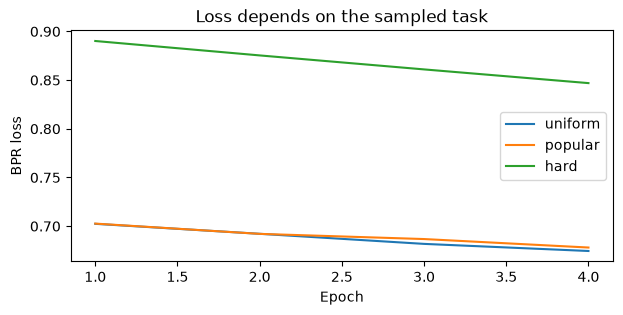
同一个mean编码器,比较均匀、训练频率^.75、16候选中取模型最高分的hard负例。屏蔽当前正例和因果前缀;未知的未来正例可能成为假负例。所有臂使用相同样本、批次顺序、初始化种子和优化预算。不同负例分布的loss不可直接比较。
PYTHON · 02
means=frame[frame.encoder=='mean'].groupby('sampler')[['ndcg@20','recall@20','coverage@20']].agg(['mean','std'])
display(means)
fig,ax=plt.subplots(figsize=(7,3))
for row in experiment['rows']:
    if row['encoder']=='mean' and row['seed']==42: ax.plot(range(1,len(row['loss'])+1),row['loss'],label=row['sampler'])
ax.set(xlabel='Epoch',ylabel='BPR loss',title='Loss depends on the sampled task');ax.legend();plt.show()
Notebook 保存的输出 · 本页未执行
| ndcg@20 | recall@20 | coverage@20 | ||||
|---|---|---|---|---|---|---|
| mean | std | mean | std | mean | std | |
| sampler | ||||||
| hard | 0.003361 | 0.002656 | 0.005247 | 0.004528 | 0.2782 | 0.022062 |
| popular | 0.003374 | 0.000790 | 0.005194 | 0.000051 | 0.4341 | 0.015415 |
| uniform | 0.004466 | 0.003811 | 0.004994 | 0.003580 | 0.3532 | 0.003111 |
<Figure size 700x300 with 1 Axes>
2 · 序列:参数量与顺序都要看
比较mean、GRU、带位置编码的自注意力池化;这是教学序列编码器,不是SASRec或DIN完整论文复现。GRU对左padding做pack处理,注意力屏蔽padding。模型没有用户ID特征。
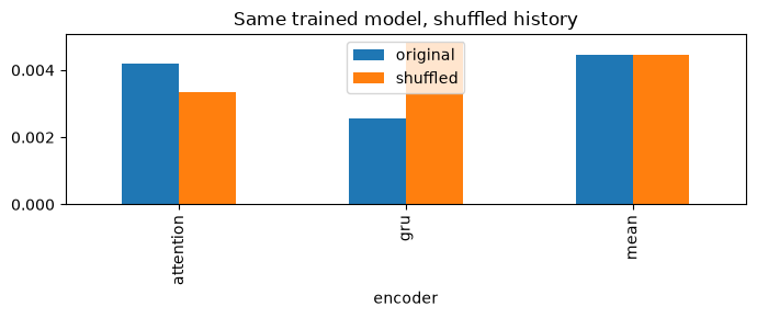
同一模型再打乱历史做推理消融;这衡量对顺序的敏感性,不证明顺序带来因果收益。两个种子也不足以声称统计显著。
PYTHON · 03
uniform=frame[frame.sampler=='uniform']
display(uniform.groupby('encoder')[['ndcg@20','recall@20','parameters']].mean())
shuffle=pd.DataFrame([{'encoder':r['encoder'],'seed':r['seed'],'original':r['ndcg@20'],'shuffled':r['shuffled']['ndcg@20']} for r in experiment['rows'] if r['sampler']=='uniform'])
display(shuffle)
shuffle.groupby('encoder')[['original','shuffled']].mean().plot.bar(figsize=(7,3),title='Same trained model, shuffled history');plt.tight_layout();plt.show()
Notebook 保存的输出 · 本页未执行
| ndcg@20 | recall@20 | parameters | |
|---|---|---|---|
| encoder | |||
| attention | 0.004205 | 0.004942 | 123504.0 |
| gru | 0.002546 | 0.002603 | 124224.0 |
| mean | 0.004466 | 0.004994 | 120624.0 |
| encoder | seed | original | shuffled | |
|---|---|---|---|---|
| 0 | mean | 42 | 0.007160 | 0.007160 |
| 1 | gru | 42 | 0.002641 | 0.006853 |
| 2 | attention | 42 | 0.004672 | 0.003519 |
| 3 | mean | 2026 | 0.001771 | 0.001771 |
| 4 | gru | 2026 | 0.002450 | 0.002790 |
| 5 | attention | 2026 | 0.003738 | 0.003169 |
<Figure size 700x300 with 1 Axes>
3 · 索引:分开看模型召回和检索近似
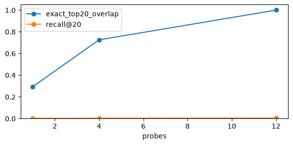
复用课程中的12簇粗索引,probes=1/4/12。记录扫描量、对精确Top20的重合率、真实标签Recall/NDCG。扫描12簇应退化到精确检索;小词表上不预设近似方法更快。
PYTHON · 04
index=pd.DataFrame([{'seed':r['seed'],**i} for r in experiment['rows'] for i in r.get('index',[])])
assert (index[index.probes==12].exact_top20_overlap==1).all()
display(index)
index.groupby('probes')[['exact_top20_overlap','recall@20']].mean().plot(marker='o',figsize=(7,3));plt.ylim(0,1.05);plt.show()
Notebook 保存的输出 · 本页未执行
| seed | probes | exact_top20_overlap | mean_scanned | seconds | recall@20 | ndcg@20 | mrr@20 | hit_rate@20 | |
|---|---|---|---|---|---|---|---|---|---|
| 0 | 42 | 1 | 0.287463 | 421.404130 | 0.034856 | 0.002371 | 0.002808 | 0.005616 | 0.026549 |
| 1 | 42 | 4 | 0.708997 | 1673.713864 | 0.079289 | 0.006380 | 0.007160 | 0.012372 | 0.032448 |
| 2 | 42 | 12 | 1.000000 | 5000.000000 | 0.185076 | 0.007526 | 0.007160 | 0.010735 | 0.035398 |
| 3 | 2026 | 1 | 0.301622 | 407.519174 | 0.034720 | 0.002246 | 0.002125 | 0.004994 | 0.026549 |
| 4 | 2026 | 4 | 0.743215 | 1643.324484 | 0.078714 | 0.001008 | 0.001674 | 0.005415 | 0.020649 |
| 5 | 2026 | 12 | 1.000000 | 5000.000000 | 0.194151 | 0.002463 | 0.001771 | 0.003196 | 0.020649 |
<Figure size 700x300 with 1 Axes>
4 · 你来改一个变量
先记录预测,再改变Config中的history、dim、epochs或samples之一,运行新实验,再重跑本章。实验会新建目录,旧权重不覆盖。比较结果要同时看预算、参数量、热门偏置与覆盖率;正式旧双塔和竞赛流程保持独立可用。
PYTHON · 05
from reclab.deep_recommendation import Config, SequenceEncoder, negatives
import inspect
print(inspect.getsource(negatives))
assert len(experiment['rows'])==len(receipt['config']['seeds'])*5
assert all(len(r['loss'])==receipt['config']['epochs'] for r in experiment['rows'])
print('PASS: complete controls and index parity checked')
Notebook 保存的输出 · 本页未执行
def negatives(history, positives, probability, rng, width=1):
    # Only causal prefix and current target are excluded. Unknown future positives remain unknown.
    out = rng.choice(len(probability), size=(len(history), width), p=probability)
    blocked = [set(row) | {int(pos), 0} for row, pos in zip(history, positives)]
    if any(sum(probability[i] for i in b) >= 1 - 1e-12 for b in blocked):
        raise ValueError('No negative support')
    for row, excluded in enumerate(blocked):
        for _ in range(100):
            bad = np.isin(out[row], list(excluded))
            if not bad.any():
                break
            out[row, bad] = rng.choice(len(probability), size=int(bad.sum()), p=probability)
        else:
            raise RuntimeError('Negative sampling failed')
    return out

PASS: complete controls and index parity checked