Retrieval, samples, and indexes
Goal
Turn concepts into inspectable inputs, operations, gradients, and comparisons.
Evidence: real snapshots + mechanism exercises. Local teaching parameters are not production defaults; mechanism experiments are not full reproductions of the original papers.
English companion. All instructional Markdown is translated. Experiment code, Chinese language examples, execution counts, and saved outputs remain as in the source edition; historical output text may therefore be Chinese. The initial setup cell anchors the working directory and Python import path for this companion's deeper folder; it does not change the experiment. Saved outputs are historical evidence, not a new run. Run from the top after preparing the required data and models.
# English companions live one directory deeper; keep the original experiment code unchanged.
from pathlib import Path as _TranslationPath
import os as _translation_os
import sys as _translation_sys
_translation_root = next((p for p in [_TranslationPath.cwd(), *_TranslationPath.cwd().parents]
                          if (p / "reclab").is_dir()), None)
if _translation_root is None:
    raise RuntimeError("Open this notebook from inside the Search Recommendation Ads Lab checkout.")
_translation_os.chdir(_translation_root)
if str(_translation_root) not in _translation_sys.path:
    _translation_sys.path.insert(0, str(_translation_root))
Setup
On the first pass, run from Setup in order: later cells reuse earlier variables. Then change one parameter and rerun that cell and its downstream cells. Constructed data does not establish real business impact.
from pathlib import Path
import sys
import inspect
import numpy as np
import pandas as pd
import matplotlib.pyplot as plt
from IPython.display import display, Code

PROJECT = next(p for p in [Path.cwd(), *Path.cwd().parents]
               if (p / "reclab/models.py").exists())
if str(PROJECT) not in sys.path:
    sys.path.insert(0, str(PROJECT))
from reclab.data import Dataset
from reclab.paths import ARTIFACTS, PROCESSED, read_json

plt.rcParams.update({"figure.figsize": (9, 3.8), "font.size": 11,
    "axes.spines.top": False, "axes.spines.right": False,
    "axes.labelcolor": "#182b2b", "text.color": "#182b2b",
    "axes.facecolor": "white", "figure.facecolor": "white",
    "grid.color": "#d4ddda", "axes.axisbelow": True})
dataset = Dataset()
print("Project:", PROJECT)
print("Dataset version:", dataset.manifest["dataset_version"])
print("Python:", sys.executable)
assert Path(sys.executable).parent == PROJECT / ".venv/bin", "请选择 Recommendation Lab 内核"
Saved notebook output · not executed on this page
Project: /Users/lizuolin/local/recommendation-lab
Dataset version: 2772cab0aca8cb81
Python: /Users/lizuolin/local/recommendation-lab/.venv/bin/python
Steps
Lecture references: 02_Retrieval_01.pdf, 02_Retrieval_02.pdf, 02_Retrieval_03.pdf, 02_Retrieval_04.pdf, 02_Retrieval_05.pdf, 02_Retrieval_06.pdf, 02_Retrieval_07.pdf, 02_Retrieval_08.pdf, 02_Retrieval_09.pdf, 02_Retrieval_10.pdf, 02_Retrieval_11.pdf, 02_Retrieval_12.pdf
UserCF and Swing
A constructed matrix you can calculate by hand. This teaching Swing variant has no user weights and counts each unordered user pair once. See notebook 01 for real ItemCF.
Predict first: If two users share ten additional liked items, does that pair's Swing contribution increase or decrease?
from reclab.learning.retrieval import (binary_matrix, usercf, swing,
    MatrixFactorization, objective_losses, kmeans, partition_retrieval,
    beam_search, SideInfoEncoder, mask_fields)
import torch
from torch.nn import functional as F
torch.set_num_threads(4); torch.manual_seed(42)
matrix = binary_matrix([(0,0),(0,1),(0,2),(1,0),(1,1),(1,2),(2,0),(2,1),(3,2),(3,3)],4,4)
display(pd.DataFrame(matrix))
display(Code(inspect.getsource(swing),language="python"))
display(pd.DataFrame(swing(matrix)))
score, neighbors, similarity = usercf(matrix,0,2)
display(pd.DataFrame({"neighbor":neighbors,"cosine":similarity}))
assert np.allclose(swing(matrix),swing(matrix).T)
Saved notebook output · not executed on this page
| 0 | 1 | 2 | 3 | |
|---|---|---|---|---|
| 0 | 1.0 | 1.0 | 1.0 | 0.0 |
| 1 | 1.0 | 1.0 | 1.0 | 0.0 |
| 2 | 1.0 | 1.0 | 0.0 | 0.0 |
| 3 | 0.0 | 0.0 | 1.0 | 1.0 |
def swing(matrix, alpha=1.0):
    """Unweighted Swing teaching variant. Each unordered user-pair is counted once."""
    if alpha <= 0:
        raise ValueError("alpha must be positive")
    histories = [set(np.flatnonzero(row)) for row in matrix]
    result = np.zeros((matrix.shape[1], matrix.shape[1]), dtype=float)
    for u, v in combinations(range(len(histories)), 2):
        common = histories[u] & histories[v]
        contribution = 1 / (alpha + len(common))
        for i, j in combinations(sorted(common), 2):
            result[i, j] += contribution
            result[j, i] += contribution
return result| 0 | 1 | 2 | 3 | |
|---|---|---|---|---|
| 0 | 0.000000 | 0.916667 | 0.25 | 0.0 |
| 1 | 0.916667 | 0.000000 | 0.25 | 0.0 |
| 2 | 0.250000 | 0.250000 | 0.00 | 0.0 |
| 3 | 0.000000 | 0.000000 | 0.00 | 0.0 |
| neighbor | cosine | |
|---|---|---|
| 0 | 1 | 1.000000 |
| 1 | 2 | 0.816497 |
Matrix factorization / BPR on real training interactions
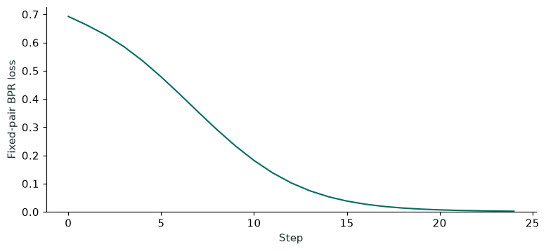
Use training-period interactions only. Fixed sampled negatives may include latent interests; lower training loss does not imply better validation quality.
Predict first: How do parameter count and fitting capacity change when dimension drops from 12 to 4?
pairs = dataset.train[["user_idx","item_idx"]].drop_duplicates().head(1500).to_numpy()
u = torch.tensor(pairs[:,0],dtype=torch.long); p = torch.tensor(pairs[:,1],dtype=torch.long)
n = torch.randint(1,dataset.n_items,(len(pairs),))
n = torch.where(n==p, n%(dataset.n_items-1)+1, n)
mf = MatrixFactorization(dataset.n_users,dataset.n_items,dim=12)
opt = torch.optim.Adam(mf.parameters(),lr=.03); curve=[]
for step in range(25):
    opt.zero_grad(); loss=mf.bpr_loss(u,p,n)
    loss.backward(); opt.step(); curve.append(float(loss.detach()))
assert curve[-1] < curve[0]
display(Code(inspect.getsource(MatrixFactorization),language="python"))
plt.plot(curve,color="#006e60"); plt.xlabel("Step"); plt.ylabel("Fixed-pair BPR loss"); plt.ylim(bottom=0); plt.show()
Saved notebook output · not executed on this page
class MatrixFactorization(nn.Module):
    def __init__(self, n_users, n_items, dim=12):
        super().__init__()
        self.users = nn.Embedding(n_users, dim)
        self.items = nn.Embedding(n_items, dim)
        nn.init.normal_(self.users.weight, std=0.1)
        nn.init.normal_(self.items.weight, std=0.1)

    def forward(self, users, items):
        return (self.users(users) * self.items(items)).sum(-1)

    def bpr_loss(self, users, positive, negative):
        return F.softplus(-(self(users, positive) - self(users, negative))).mean()
<Figure size 900x380 with 1 Axes>
Three losses, sampling exponents, and LogQ
Loss magnitudes are not comparable across definitions. The lectures' 50/50 hard-negative recipe requires logs of candidates rejected by ranking, which this dataset lacks.
Predict first: What happens to the probability of sampling a popular item when the exponent is 0 or 1?
p=torch.tensor([1.,2.,.5],requires_grad=True); n=torch.tensor([0.,1.,1.],requires_grad=True)
display(pd.Series({k:float(v.detach()) for k,v in objective_losses(p,n).items()}).to_frame("loss"))
counts=np.array([1.,10.,100.,1000.]); exponent=.75
sampling=counts**exponent; sampling/=sampling.sum()
display(pd.DataFrame({"count":counts,"uniform":.25,"power_sampling":sampling,"in_batch_prior":counts/counts.sum()}))
logits=torch.ones(1,4)
display(pd.DataFrame({"raw":logits.softmax(-1)[0].numpy(),
    "logq_corrected":(logits-torch.log(torch.tensor(sampling))[None,:]).softmax(-1)[0].numpy()}))
Saved notebook output · not executed on this page
| loss | |
|---|---|
| pointwise | 0.705656 |
| pairwise | 0.533533 |
| listwise | 0.533533 |
| count | uniform | power_sampling | in_batch_prior | |
|---|---|---|---|---|
| 0 | 1.0 | 0.25 | 0.004628 | 0.000900 |
| 1 | 10.0 | 0.25 | 0.026025 | 0.009001 |
| 2 | 100.0 | 0.25 | 0.146352 | 0.090009 |
| 3 | 1000.0 | 0.25 | 0.822995 | 0.900090 |
| raw | logq_corrected | |
|---|---|---|
| 0 | 0.25 | 0.822995 |
| 1 | 0.25 | 0.146352 |
| 2 | 0.25 | 0.026025 |
| 3 | 0.25 | 0.004628 |
Real item-vector caches and partition-based approximate retrieval
Overlap with exact top 20 measures index error, not recall of user preferences. No large-scale ANN system is deployed.
Predict first: Why do more probes usually increase cost? How should cache versions be paired for full and incremental updates?
vectors=np.load(ARTIFACTS/"runs/baseline-history32/item_vectors.npy")[1:]
query=vectors[0]; exact=np.argsort(-(vectors@query))[:20]
centers, labels=kmeans(vectors,clusters=12,iterations=5)
rows=[]
for probes in [1,3,6,12]:
    found,count=partition_retrieval(vectors,query,centers,labels,probes=probes,k=20)
    rows.append({"probes":probes,"scored":count,"exact_top20_overlap":len(set(found)&set(exact))/20})
display(pd.DataFrame(rows))
assert rows[-1]["exact_top20_overlap"]==1.
Saved notebook output · not executed on this page
| probes | scored | exact_top20_overlap | |
|---|---|---|---|
| 0 | 1 | 325 | 0.35 |
| 1 | 3 | 1122 | 1.00 |
| 2 | 6 | 2609 | 1.00 |
| 3 | 12 | 5000 | 1.00 |
The path-search component of Deep Retrieval
Only conditional path probabilities and beam search are reproduced. Neural path learning and alternating optimization are absent; this is not full Deep Retrieval.
Predict first: Why can the locally highest probability fail to produce the highest-probability complete path?
transition={():{"A":.6,"B":.4},("A",):{"x":.5,"y":.5},("B",):{"x":.99,"y":.01}}
display(Code(inspect.getsource(beam_search),language="python"))
display(pd.DataFrame([{"width":w,"best":beam_search(transition,width=w)[0][0],
    "probability":np.exp(beam_search(transition,width=w)[0][1])} for w in [1,2,4]]))
assert beam_search(transition,width=1)[0][0] != beam_search(transition,width=4)[0][0]
Saved notebook output · not executed on this page
def beam_search(transition, depth=2, width=1):
    """Conditional path probabilities. No neural path/index learning is claimed."""
    beams = [((), 0.0)]
    for _ in range(depth):
        expanded = []
        for path, log_prob in beams:
            for node, probability in transition[path].items():
                expanded.append((path + (node,), log_prob + np.log(probability)))
        beams = sorted(expanded, key=lambda row: (-row[1], row[0]))[:width]
return beams| width | best | probability | |
|---|---|---|---|
| 0 | 1 | (A, x) | 0.300 |
| 1 | 2 | (B, x) | 0.396 |
| 2 | 4 | (B, x) | 0.396 |
Field self-supervision and Bloom filters
Use real attributes available at the training cutoff to inspect SSL gradients. The auxiliary task is not connected to the main two-tower trainer. Bloom filters use constructed integer IDs, not real impression logs.
Predict first: What changes when Bloom-filter storage doubles? How does masking a field differ from hidden-layer dropout?
cats={v:i+1 for i,v in enumerate(sorted({x["category"] for x in dataset.items}))}
ids=torch.arange(1,65); categories=torch.tensor([cats[x["category"]] for x in dataset.items[:64]])
encoder=SideInfoEncoder(dataset.n_items,len(cats)+1)
a=encoder(*mask_fields(ids,categories,.5)); b=encoder(*mask_fields(ids,categories,.5))
ssl=F.cross_entropy(a@b.T/.2,torch.arange(64)); ssl.backward()
assert torch.isfinite(ssl)
print("SSL mechanism loss:",float(ssl.detach()))
from reclab.learning.systems import BloomFilter
bloom=BloomFilter(bits=512,hashes=4)
for i in range(100):bloom.add(i)
assert all(bloom.contains(i) for i in range(100))
print("False positives on 5000 unseen IDs:",np.mean([bloom.contains(i) for i in range(100,5100)]))
print("Author/geo/social retrieval requires matching fields; see explicitly simulated social exercise in chapter 10.")
Saved notebook output · not executed on this page
SSL mechanism loss: 3.8621013164520264
False positives on 5000 unseen IDs: 0.093
Author/geo/social retrieval requires matching fields; see explicitly simulated social exercise in chapter 10.
Checks
Every assertion and output is traceable to code. They check operators, data snapshots, or mechanisms, not online gains.
Next steps
Record your prediction, change only one variable, and run the relevant experiment cell. Open reclab/learning/ to inspect helper functions.