02 · 双塔:源码、张量、梯度与真实训练
Goal
从可编辑的 Python 网络走到真实训练。你可以改维度、历史窗口、学习率,也可以在左侧文件浏览器中打开 reclab/models.py 修改正式网络。
Run All 会在最后创建一个新模型版本,保留原来的数据和模型。本教程先做小 Batch 数学检查,再运行项目的共享训练器;不使用测试集。
Setup
使用项目的 Recommendation Lab (Python 3.12) 内核。下面的用户和物品来自现有真实训练集;小 Batch 实验只是检查梯度,不能证明推荐效果提升。
from pathlib import Path
import sys
import inspect
import numpy as np
import pandas as pd
import matplotlib.pyplot as plt
from IPython.display import display, Code

PROJECT = next(p for p in [Path.cwd(), *Path.cwd().parents]
               if (p / "reclab/models.py").exists())
if str(PROJECT) not in sys.path:
    sys.path.insert(0, str(PROJECT))
from reclab.data import Dataset
from reclab.paths import ARTIFACTS, PROCESSED, read_json

plt.rcParams.update({"figure.figsize": (9, 3.8), "font.size": 11,
    "axes.spines.top": False, "axes.spines.right": False,
    "axes.labelcolor": "#182b2b", "text.color": "#182b2b",
    "axes.facecolor": "white", "figure.facecolor": "white",
    "grid.color": "#d4ddda", "axes.axisbelow": True})
dataset = Dataset()
print("Project:", PROJECT)
print("Dataset version:", dataset.manifest["dataset_version"])
print("Python:", sys.executable)
assert Path(sys.executable).parent == PROJECT / ".venv/bin", "请选择 Recommendation Lab 内核"
Notebook 保存的输出 · 本页未执行
Project: /Users/lizuolin/local/recommendation-lab
Dataset version: 2772cab0aca8cb81
Python: /Users/lizuolin/local/recommendation-lab/.venv/bin/python
import torch
from torch import nn
from torch.nn import functional as F
import reclab.models as model_module
from reclab.models import TwoTower
torch.set_num_threads(4)
torch.manual_seed(42)
DIM = 32
HISTORY_LEN = 20
BATCH = 8
TEMPERATURE = 0.1
Steps
1. 直接看当前网络源码
这就是网页服务使用的类。要修改它,在左侧打开 reclab/models.py;保存后重启内核再从头执行,或使用最后训练格中的模块 reload。
print(inspect.getfile(TwoTower))
display(Code(inspect.getsource(TwoTower), language="python"))
Notebook 保存的输出 · 本页未执行
/Users/lizuolin/local/recommendation-lab/reclab/models.py
class TwoTower(nn.Module):
    def __init__(self, n_users, n_items, dim=32, use_history=True, dropout=0.1):
        super().__init__()
        self.use_history = use_history
        self.user_embedding = nn.Embedding(n_users, dim)
        self.item_embedding = nn.Embedding(n_items, dim, padding_idx=0)
        self.user_mlp = nn.Sequential(
            nn.Linear(dim * 2, dim * 2),
            nn.ReLU(),
            nn.Dropout(dropout),
            nn.Linear(dim * 2, dim),
        )
        self.item_mlp = nn.Sequential(
            nn.Linear(dim, dim * 2), nn.ReLU(), nn.Linear(dim * 2, dim)
        )

    def encode_user(self, users, history):
        mask = (history != 0).unsqueeze(-1)
        pooled = (self.item_embedding(history) * mask).sum(1) / mask.sum(1).clamp_min(1)
        if not self.use_history:
            pooled = torch.zeros_like(pooled)
        return F.normalize(
            self.user_mlp(torch.cat([self.user_embedding(users), pooled], dim=-1)),
            dim=-1,
        )

    def encode_item(self, items):
        return F.normalize(self.item_mlp(self.item_embedding(items)), dim=-1)

    def loss(self, users, history, targets, temperature=0.1, logq=None):
        # In-batch sampled softmax. Duplicate positive IDs are accidental hits, not negatives.
        logits = (
            self.encode_user(users, history) @ self.encode_item(targets).T / temperature
        )
        if logq is not None:
            logits = logits - logq[targets][None, :]
        duplicate = targets[:, None].eq(targets[None, :])
        duplicate.fill_diagonal_(False)
        logits = logits.masked_fill(duplicate, -1e9)
        return F.cross_entropy(logits, torch.arange(len(users), device=users.device))
2. 用真实样本追踪张量形状
用户 [B]、历史 [B,N]、目标 [B]。两侧编码后都是 [B,D];用户向量乘目标向量转置得到 [B,B]。
users_np, histories_np, targets_np, times_np = dataset.examples(HISTORY_LEN)
users = torch.from_numpy(users_np[:BATCH])
histories = torch.from_numpy(histories_np[:BATCH])
targets = torch.from_numpy(targets_np[:BATCH])
model = TwoTower(dataset.n_users, dataset.n_items, dim=DIM, use_history=True, dropout=0.0)
model.eval()  # 固定本次数学诊断;eval 不等于关闭 autograd
user_vectors = model.encode_user(users, histories)
item_vectors = model.encode_item(targets)
display(pd.DataFrame({"tensor": ["users", "histories", "targets", "user_vectors", "item_vectors"],
    "shape": [list(x.shape) for x in [users, histories, targets, user_vectors, item_vectors]]}))
print("Trainable parameters:", sum(p.numel() for p in model.parameters()))
assert torch.allclose(user_vectors.norm(dim=1), torch.ones(BATCH), atol=1e-6)
Notebook 保存的输出 · 本页未执行
| tensor | shape | |
|---|---|---|
| 0 | users | [8] |
| 1 | histories | [8, 20] |
| 2 | targets | [8] |
| 3 | user_vectors | [8, 32] |
| 4 | item_vectors | [8, 32] |
Trainable parameters: 385952
3. 把 sampled softmax 损失展开
先预测:降低温度会让分布更尖锐,还是更平滑?
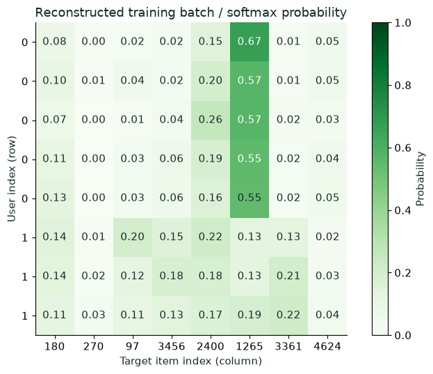
每行的正确类别在对角线。其他目标是 batch 内采样负例,重复目标会屏蔽。这里不启用 LogQ,便于先核对基本数学;它们并不是真实“曝光未点击”。
cosine = user_vectors @ item_vectors.T
duplicate = targets[:, None].eq(targets[None, :])
duplicate.fill_diagonal_(False)
logits = (cosine / TEMPERATURE).masked_fill(duplicate, -1e9)
logits.retain_grad()
labels = torch.arange(BATCH)
probabilities = logits.softmax(dim=1)
loss = F.cross_entropy(logits, labels)
model.zero_grad(set_to_none=True)
loss.backward()
expected_gradient = (probabilities.detach() - F.one_hot(labels, BATCH)) / BATCH
assert torch.allclose(logits.grad, expected_gradient, atol=1e-6)
display(pd.DataFrame(probabilities.detach().numpy(), index=users.tolist(), columns=targets.tolist()))
print("Cross-entropy:", float(loss.detach()))
print("dL/dlogit for row 0:", logits.grad[0].tolist())
Notebook 保存的输出 · 本页未执行
| 180 | 270 | 97 | 3456 | 2400 | 1265 | 3361 | 4624 | |
|---|---|---|---|---|---|---|---|---|
| 0 | 0.075222 | 0.004755 | 0.016481 | 0.023495 | 0.147182 | 0.670796 | 0.012573 | 0.049495 |
| 0 | 0.097509 | 0.006899 | 0.040241 | 0.024322 | 0.198824 | 0.573799 | 0.008774 | 0.049632 |
| 0 | 0.067674 | 0.002751 | 0.012127 | 0.037660 | 0.259269 | 0.570432 | 0.022318 | 0.027770 |
| 0 | 0.109721 | 0.001928 | 0.027018 | 0.061421 | 0.187387 | 0.552615 | 0.017557 | 0.042352 |
| 0 | 0.127011 | 0.002267 | 0.028390 | 0.062393 | 0.160158 | 0.546719 | 0.018724 | 0.054338 |
| 1 | 0.144987 | 0.011143 | 0.200329 | 0.150079 | 0.215864 | 0.127405 | 0.128882 | 0.021311 |
| 1 | 0.135188 | 0.015927 | 0.120577 | 0.184901 | 0.181037 | 0.128408 | 0.208228 | 0.025733 |
| 1 | 0.114495 | 0.027263 | 0.112846 | 0.134311 | 0.165850 | 0.189183 | 0.218638 | 0.037414 |
Cross-entropy: 2.9391064643859863
dL/dlogit for row 0: [-0.115597203373909, 0.0005943385185673833, 0.002060179365798831, 0.002936860080808401, 0.01839778758585453, 0.08384954929351807, 0.00157161767128855, 0.006186868529766798]
fig, ax = plt.subplots(figsize=(7.5, 5.5))
image = ax.imshow(probabilities.detach().numpy(), cmap="Greens", vmin=0, vmax=1)
ax.set_xticks(range(BATCH), [str(i) for i in targets.tolist()])
ax.set_yticks(range(BATCH), [str(i) for i in users.tolist()])
ax.set(xlabel="Target item index (column)", ylabel="User index (row)",
       title="Reconstructed training batch / softmax probability")
for row in range(BATCH):
    for col in range(BATCH):
        value = float(probabilities[row, col].detach())
        text = "x" if duplicate[row, col] else f"{value:.2f}"
        ax.text(col, row, text, ha="center", va="center", color="white" if value > .55 else "#182b2b")
fig.colorbar(image, ax=ax, label="Probability")
plt.tight_layout(); plt.show()
Notebook 保存的输出 · 本页未执行
<Figure size 750x550 with 2 Axes>
4. 先让一个小 Batch 过拟合
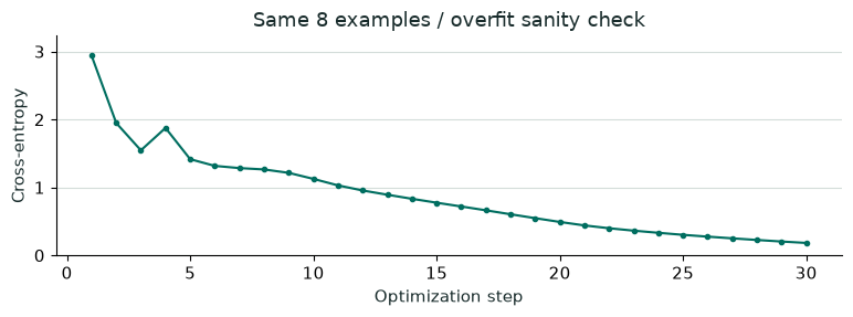
这是训练代码的 sanity check。只更新 Notebook 内存中的新模型,不覆盖已保存的权重;小 Batch loss 下降不代表验证指标提高。
optimizer = torch.optim.Adam(model.parameters(), lr=0.01)
tiny_losses = []
for step in range(30):
    optimizer.zero_grad(set_to_none=True)
    tiny_loss = model.loss(users, histories, targets, TEMPERATURE)
    tiny_losses.append(float(tiny_loss.detach()))
    tiny_loss.backward()
    optimizer.step()
assert tiny_losses[-1] < tiny_losses[0]
print("Tiny-batch loss:", tiny_losses[0], "->", tiny_losses[-1])
fig, ax = plt.subplots(figsize=(8, 3))
ax.plot(range(1,31), tiny_losses, color="#006e60", marker=".")
ax.set(xlabel="Optimization step", ylabel="Cross-entropy", title="Same 8 examples / overfit sanity check", ylim=(0, max(tiny_losses)*1.1))
ax.grid(axis="y"); plt.tight_layout(); plt.show()
Notebook 保存的输出 · 本页未执行
Tiny-batch loss: 2.9391064643859863 -> 0.18255160748958588
<Figure size 800x300 with 1 Axes>
5. 在本格里试着改网络
MyTwoTower 是一个独立学习分支,只检查前向传播。把 ReLU 换成 Tanh,或改 HIDDEN,观察参数量和输出形状。
这一格没有替换正式训练器。希望工作台使用新结构时,编辑真实的 reclab/models.py,然后运行下面的完整训练格。
HIDDEN = 16
class MyTwoTower(TwoTower):
    def __init__(self, n_users, n_items, dim):
        super().__init__(n_users, n_items, dim, use_history=True, dropout=0.0)
        self.user_mlp = nn.Sequential(nn.Linear(2*dim, HIDDEN), nn.ReLU(), nn.Linear(HIDDEN, dim))

sandbox = MyTwoTower(dataset.n_users, dataset.n_items, DIM)
print("Edited user tower:", sandbox.user_mlp)
print("Output shape:", tuple(sandbox.encode_user(users, histories).shape))
print("Parameters:", sum(p.numel() for p in sandbox.parameters()))
Notebook 保存的输出 · 本页未执行
Edited user tower: Sequential(
  (0): Linear(in_features=64, out_features=16, bias=True)
  (1): ReLU()
  (2): Linear(in_features=16, out_features=32, bias=True)
)
Output shape: (8, 32)
Parameters: 381296
6. 跑项目真实训练器,保存新版本
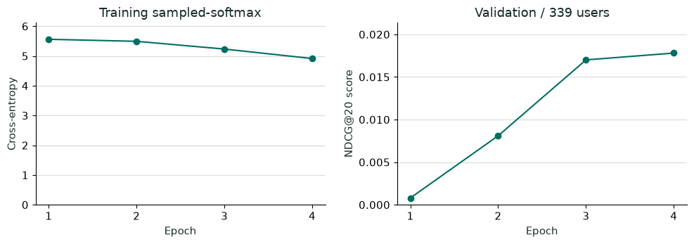
先只改 EXPERIMENT 中一个变量。保存后的模型、配置、曲线会出现在网页“训练与实验”里(刷新页面)。它使用完整训练子集和固定验证口径,不使用上面的 8 条样本作为评估。
reload 会读取你已经保存的 models.py / train.py。修改结构后从新模型开始训练;不要用不兼容的新结构加载旧 checkpoint。
import importlib
import reclab.train as train_module
importlib.reload(model_module)
train_module = importlib.reload(train_module)

EXPERIMENT = train_module.TrainConfig(
    name="notebook / first-full-run", dim=32, history_len=20,
    epochs=4, batch_size=256, learning_rate=0.003,
    use_history=True, logq_correction=False, seed=42,
)
new_run = train_module.train(EXPERIMENT)
print("Saved run:", new_run["run_id"])
display(pd.Series(new_run["validation"]["metrics"], name="validation score").to_frame())
Notebook 保存的输出 · 本页未执行
20261028T023407346105 {'epoch': 1, 'loss': 5.560806380245401, 'gradient_norm_before_clip': 0.3162150839824632, 'validation_ndcg@20': 0.0007904414175060725, 'validation_recall@20': 0.000609776941282452, 'elapsed_seconds': 1.81}
20261028T023407346105 {'epoch': 2, 'loss': 5.492199623965221, 'gradient_norm_before_clip': 0.32834317195863233, 'validation_ndcg@20': 0.008092865280543902, 'validation_recall@20': 0.014427202969790203, 'elapsed_seconds': 2.38}
20261028T023407346105 {'epoch': 3, 'loss': 5.232908364200719, 'gradient_norm_before_clip': 0.5570250882509169, 'validation_ndcg@20': 0.01700333691787301, 'validation_recall@20': 0.031168373965094427, 'elapsed_seconds': 2.93}
20261028T023407346105 {'epoch': 4, 'loss': 4.913768497700725, 'gradient_norm_before_clip': 0.7106661569904273, 'validation_ndcg@20': 0.017804264366807675, 'validation_recall@20': 0.03713369853338916, 'elapsed_seconds': 3.53}
Saved run: 20261028T023407346105
| validation score | |
|---|---|
| recall@10 | 0.028066 |
| ndcg@10 | 0.014543 |
| mrr@10 | 0.011672 |
| hit_rate@10 | 0.038348 |
| recall@20 | 0.037134 |
| ndcg@20 | 0.017804 |
| mrr@20 | 0.013524 |
| hit_rate@20 | 0.064897 |
| recall@50 | 0.071146 |
| ndcg@50 | 0.025709 |
| mrr@50 | 0.015489 |
| hit_rate@50 | 0.126844 |
| recall@100 | 0.092180 |
| ndcg@100 | 0.030524 |
| mrr@100 | 0.016271 |
| hit_rate@100 | 0.185841 |
| catalog_coverage@20 | 0.563400 |
curve = pd.DataFrame(new_run["curve"])
fig, axes = plt.subplots(1, 2, figsize=(10, 3.6))
axes[0].plot(curve.epoch, curve.loss, color="#006e60", marker="o")
axes[0].set(title="Training sampled-softmax", xlabel="Epoch", ylabel="Cross-entropy", ylim=(0, curve.loss.max()*1.1))
axes[1].plot(curve.epoch, curve["validation_ndcg@20"], color="#006e60", marker="o")
axes[1].set(title=f"Validation / {new_run['validation']['audit']['evaluated_users']} users", xlabel="Epoch", ylabel="NDCG@20 score", ylim=(0, max(curve["validation_ndcg@20"].max()*1.2, .001)))
for ax in axes:
    ax.set_xticks(curve.epoch)
    ax.grid(axis="y")
plt.tight_layout(); plt.show()
Notebook 保存的输出 · 本页未执行
<Figure size 1000x360 with 2 Axes>
Checks
本 Notebook 用断言检查了向量归一化、交叉熵梯度公式,以及真实小 Batch 能否优化。最终模型由验证 NDCG@20 选择 checkpoint,结果保存到 artifacts/runs/<run_id>/。
Next Steps
先写下预测,再仅改变 history_len 或 learning_rate 重跑完整训练格。训练 loss 和验证指标是否同向变化?用 configs/no-history.json 对照历史特征的作用。
当前机制参考双塔模型、LastN 与 batch 内负样本讲义;这不是原论文数据与工业规模的完整复现。测试集保留给最终验收,继续实验不要围绕它调参。